Excel Filter Shortcut
Written by
Reviewed by
Last updated on October 19, 2023
This tutorial will demonstrate shortcuts for creating and working with Filters in Excel.
Filters in Excel
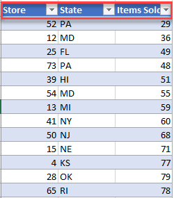
A filter is used on a set of data to customize what you want to look at. A filter allows you to select, which rows of a dataset to show. You can tell when a filter has been created, by the arrows that appear at the top of the data:
AutoFilter Shortcut
To apply a filter to a range:
- Click on the dataset
- Use the shortcut:
PC Shortcut:Ctrl+Shift+LMac Shortcut:⌘+⇧+FRemember This Shortcut:
L for Filter
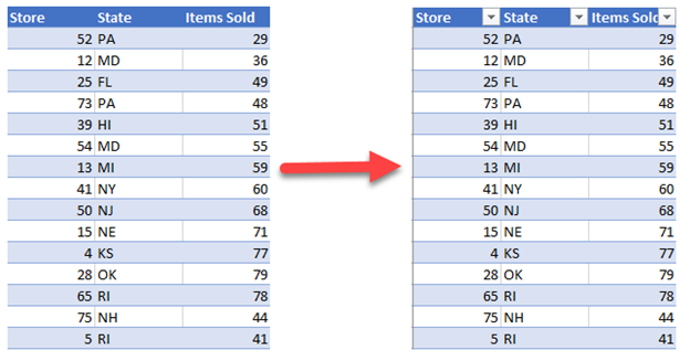
Now your filter is applied, allowing you to filter your data.
Open Filter Shortcut
Once a filter has been applied, it’s easy to activate the filter without using the mouse.
- Use the arrow keys to navigate to the header cell with the filter (look for the down arrows)
- Press (and hold):
PC Shortcut: ALT+↓Mac Shortcut: ⌥+↓
This will open up the filter dropdown.
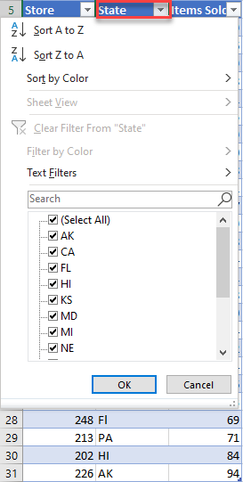
Filter Menu Shortcuts
- Use the Down / Up Arrow keys to navigate within the menu
- Use TAB to navigate down the menu
- Use SHIFT + TAB to navigate up the menu.
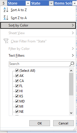
- Press SPACE within filter menu to check/uncheck filter
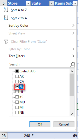
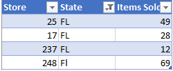
Filtered Data
When clicking OK, the data will filter to what you selected, as shown below.