Cell References – Absolute, A1, R1C1, 3D, Circular in Excel & Google Sheets
Written by
Reviewed by
In order to make accurate calculations in Excel, it’s essential to understand how the different types of cell references work.
A1 vs. R1C1 References
Excel worksheets contain many cells and (by default) each cell is identified by its column letter followed by its row number. This is known as A1-style referencing. Examples: A1, B4, C6
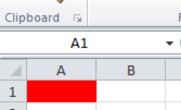
A1 reference style
Optionally, you can switch to R1C1 Reference Mode to refer to a cell’s row & column number. Instead of referring to cell A1 you would refer to R1C1 (row 1, column 1). Cell C4 would be referred to R4C3.
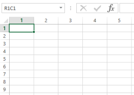
R1C1 reference style
R1C1-style referencing is extremely uncommon in Excel. Unless you have a good reason you should probably stick to the default A1-style reference mode. However, if you use VBA you will likely encounter this reference style.
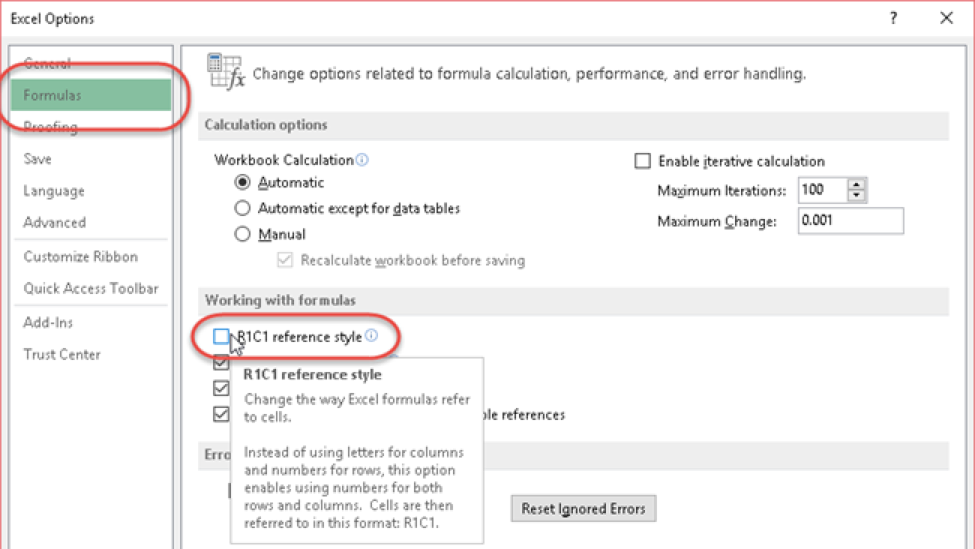
Switch to R1C1 Reference Style
To switch the reference style, go to File > Option > Formula. Check the box next to R1C1 reference style.
Named Ranges
One of the most under-utilized features of Excel is the Named Ranges feature. Instead of referring to a cell (or group of cells) by its cell location (ex B3 or R3C2), you can name that range and simply reference the range name in your formulas.
To name a range:
- Select the cell or cells that you wish to name
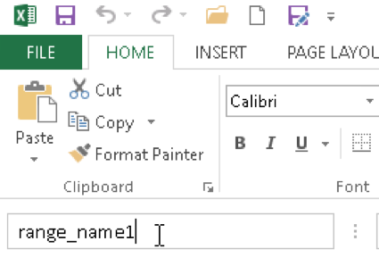
- Click Inside the Range Name Box
- Enter your desired name
- Hit Enter
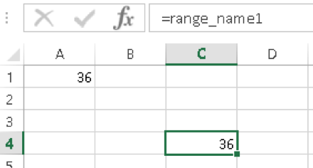
Now you can reference cell A1 by typing =range_name1 instead. This is very useful when working with large workbooks with multiple worksheets.
Range of Cells
When using Excel’s built in Functions, you may need to reference ranges of cells. Cell ranges appear like this ‘A1:B3’. This reference refers to all cells in between A1 and B3: cells A1,A2,A3, B1, B2, B3.
To select a range of cells when entering a formula:
- Type in the range (separate the start and end range with a semicolon)
- Use your mouse to click the first cell reference, hold down the mouse button and drag your desired range.
- Hold down the shift key and navigate with the arrow keys to select your range
Absolute (Frozen) and Relative References
When entering cell references within formulas, you can use relative or absolute (frozen) references. Relative references will move proportionally when you copy the formula to a new cell. Absolute references will remain unchanged. Let’s look at some examples:
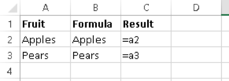
Relative Reference
A relative reference in Excel looks like this
=A1
When you copy and paste a formula with relative references, the relative references will move proportionally. Unless you specify otherwise, your cell references will be relative (unfrozen) by default.
Example: If you copy ‘=A1’ down one row the reference changes to ‘=A2’.
Absolute (Frozen) Cell References
If you don’t want your cell references to move when you copy a formula, you can “freeze” your cell references by adding dollar signs ($s) in front of the reference that you want frozen. Now when you copy and paste the formula, the cell reference will remain unchanged. You can choose to freeze the row reference, column reference, or both.
A1: Nothing is frozen
$A1: The column is frozen, but the row is not frozen
A$1: The row is frozen, but the column is not frozen
$A$1: Both the row and column are frozen
Absolute Reference Shortcut
Manually adding in dollar signs ($s) into your formulas isn’t very practical. Instead, while creating your formula, use the F4 key to toggle between absolute/relative cell references.
Absolute Cell Reference Example
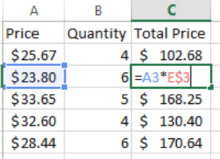
When would you actually need to freeze a cell reference? One common example is when you have input cells that are referenced frequently. In the example below, we want to calculate the sales tax for each quantity of menu items. The sales tax is constant across all items, so we will reference the sales tax cell repeatedly.
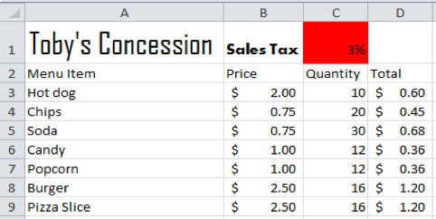
To find the total sales tax, enter the formula ‘=(B3*C3)*$C$1’ in column D and the copy the formula down.
Mixed Reference
You may have heard of mixed cell references. A mixed reference is when either the row or column reference is locked (but not both).
Mixed Reference
Remember, by using the “F4” key you are able to cycle through your relative, absolute cell references.
Cell References – Inserting & Deleting Rows/Columns
You may be wondering what happens to your cell references when you insert or delete rows/columns?
The cell reference will update automatically to refer to the original cell. This is the case regardless of whether the cell reference is frozen.
3D References
At times, you may need to work with several worksheets with identical patterns of data. Excel allows you to refer to multiple sheets at once without needing to manually enter each worksheet. You can reference a range of sheets similar to how would reference a range of cells. Example ‘Sheet1:Sheet5!A1’ would reference cells A1 on all sheets from Sheet1 to Sheet5.
Let’s walk through an example:
You want to add together the total units sold for each product across all stores. Each store has its own worksheet and all the worksheets have an identical format. You could create a formula similar to this:
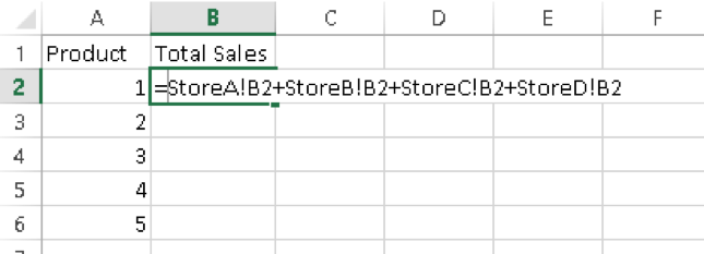
This is not too difficult with only four worksheets, but what if you had 40 worksheets? Would you really want to manually add each cell reference?
Instead, you can use a 3D reference to reference multiple sheets at once with ease(similar to how you can reference a range of cells).
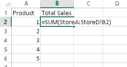
Be Careful! The order of your worksheets matters. If you move another sheet in between the referenced sheets (StoreA and StoreD) that sheet will be included. Conversely, if you move a sheet outside the range of sheets (before StoreA or after StoreD), it will no longer be included.
Circular Cell Reference
A circular cell reference is when a cell refers back to itself. For example, if the result of cell B1 is used as an input for cell B1 then a circular reference is created. The cell does not need to directly refer to itself There can be intermediate steps.
Example:
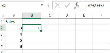
In this case, the formula for cell B2 is “A2+A3+B2”. Because you are in cell B2, you may not use B2 in the equation. This would trigger circular reference and the value in cell “B2” will automatically be set to “0”.
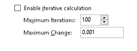
Usually circular references are a result of user error, but in there are circumstances in which you may want to use a circular reference. The primary example of using a circular reference is to calculate values iteratively. To do this, you need to go to File > Options > Formulas and Enabled Iterative Calculation:
External References
At times when calculating data you may need to refer to data outside of your workbook. This is called an external reference (link).
To select an external reference while creating a formula, navigate to the external workbook, and select your reference as you normally would.
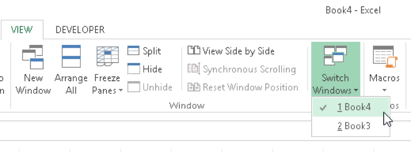
To navigate to the other workbook you can use the CTRL + TAB shortcut or go to View > Switch Windows.
Once you’ve selected the cell, you’ll see that an external reference that looks like this:
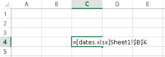
Notice that the workbook name is enclosed by brackets [].
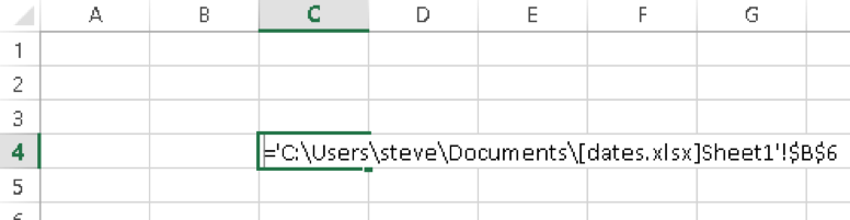
Once you close the referenced workbook, the reference will show the file location:
When you reopen the workbook containing the external link, you will be prompted to enable automatic updating of links. If you do so, then Excel will open the reference value with the current value of the workbook. Even if it’s closed! Be careful! You may or may not want this.
Named Ranges and External References
What happens to your external cell reference when rows / columns are added or deleted from the reference workbook? If both workbooks are open then the cell references update automatically. However, if both workbooks aren’t open then the cell references won’t update and will no longer be valid. This is a huge concern when linking to external workbooks. Many errors are caused by this.
If you do link to external workbooks, you should name the cell reference with a named range (see previous section for more information). Now your formula will refer to the named range no matter what changes occur on the external workbook.

