How to Create an Ogive Graph in Excel

This tutorial will demonstrate how to create an ogive graph in all versions of Excel: 2007, 2010, 2013, 2016, and 2019.

An ogive graph (also known as a cumulative frequency graph) is a graph used in statistics to illustrate cumulative frequencies, which are measured by adding each frequency (the number of observations) to the sum of the frequencies preceding it in the dataset.

In other words, the phrase “cumulative frequency” means that you are adding up values as you go along.

The purpose of the chart is to show the total number of data points in the dataset that are less than or equal to a particular value. It helps us swiftly examine how many observations (frequencies) fall into a certain range across the entire dataset.

However, as the chart is not supported in Excel, you will have to put in some work to create it from scratch. And that’s where the Chart Creator Add-in comes into play, a powerful tool for building advanced Excel charts in just a few clicks.

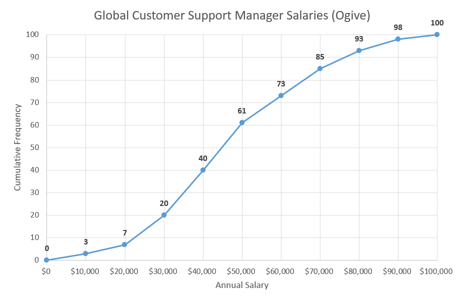
In this tutorial, you will learn how to calculate cumulative frequencies and create this ogive graph in Excel from the ground up:

Getting Started

For illustration purposes, suppose you work as a statistician at a major corporation with branches all over the world.

You have been assigned the task of analyzing the annual salaries of 100 global customer support managers across all the branches—obviously, the compensation differs from country to country.

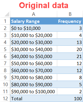
With that, you set out to plot an ogive graph using the data in the following table:

A few words on each element:

• Annual Salary Range: This categorical variable represents the class limits—or, in statistical parlance, the bins—which set the boundaries among the salary ranges. In other words, it’s how we categorize the observations.
• Frequency: This quantitative variable illustrates the number of times a given observation takes place in a dataset. In our case, it shows how many company workers earn the annual pay that falls into a certain salary range.

Now, let’s get down to work.

Step #1: Create a helper table.

First things first, set up a helper table to give you a place to compute all the chart data necessary for plotting the ogive graph.

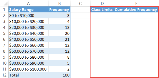
The columns in this helper table go as follows:

• Class Limits: This column will define the ogive intervals based on your actual class limits.
• Cumulative Frequency: This column will contain all the cumulative frequencies you will calculate further down the road.

Step #2: Define the class limits.

Right off the bat, let’s fill up the column labeled Class Limits (column D).

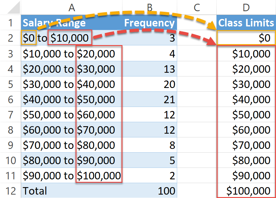
By convention, the first empty cell in the column (D2) must equal the very lowest class limit in the entire dataset (in our case, that’s $0—you can’t really go any lower than that).

Moving down the column, the subsequent cells are to be filled with the upper-class limits (the higher number) of each salary range, including the first one used to obtain the lowest class limit (A2:A11). For instance, take the salary range of $0 to $10,000 (A2).

In that case, the upper-class limit is $10,000 while the lower-class limit equals $0 (which we put into D2). You will then put $10,000 into the next cell down (D3). The next salary range is $10,000 to $20,000 (A3). You will take the upper-class limit of $20,000 and input that in D4. Continue the process down the list.

It may sound like rocket science, but in reality, the algorithm is laughingly simple. Here is how it looks in practice:

Step #3: Compute the cumulative frequencies.

Having set the intervals, it’s time to calculate the cumulative frequencies for column E.

Again, by convention, since you should always start a count from zero, type “0” into the first blank cell in the column (E3).

As for the rest, here is the one-size-fits-all formula you need to copy into cell E3 to determine the remaining values:

=SUM($B$2:B2)

This formula locks cell B2 and calculates the sum of the values within the specified range, saving you time on adding up the values on your own. Here is how it should look:

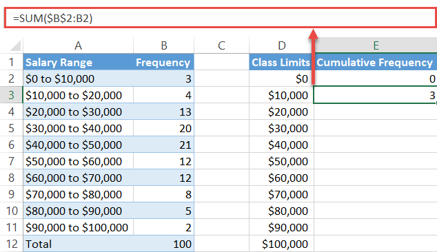
Drag the fill handle in the bottom right corner of the selected cell E3 all the way down to the bottom of column E to copy the formula into the remaining cells (E4:E12).

Step #4: Plot the ogive graph.

Finally, you can now put all the puzzle pieces together to plot the ogive graph.

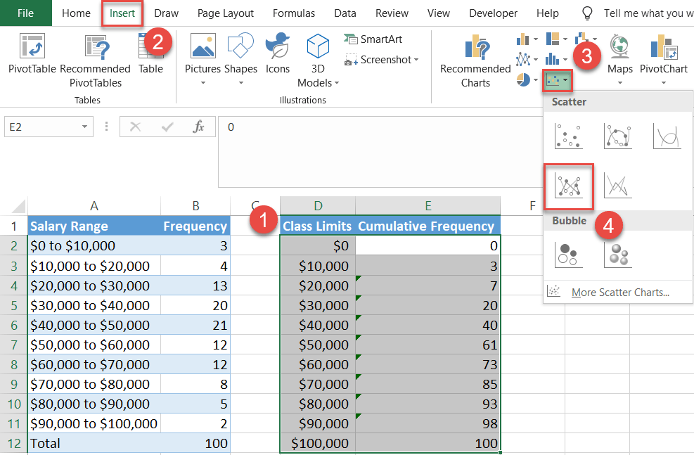
1. Highlight all the values in the helper table (columns D and E).
2. Go to the Insert tab.
3. Select the “Insert Scatter (X, Y) or Bubble Chart” button.
4. Choose “Scatter with Straight Lines and Markers.”

Step #5: Modify the horizontal axis scale.

Technically, you can stop right here, but such an ogive would be hard to read without clarifying its data by adding a few more details.

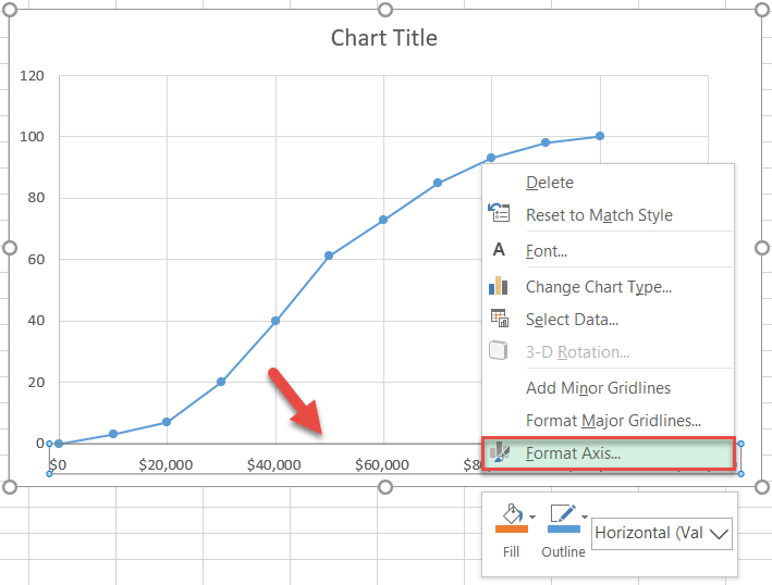
So let’s make it more informative by changing the small things that matter—like they say, the devil is in the detail. First, we will tinker with the horizontal axis scale.

Right-click on the horizontal axis (the numbers along the bottom) and pick “Format Axis” from the menu that appears.

In the task pane that pops up, do the following:

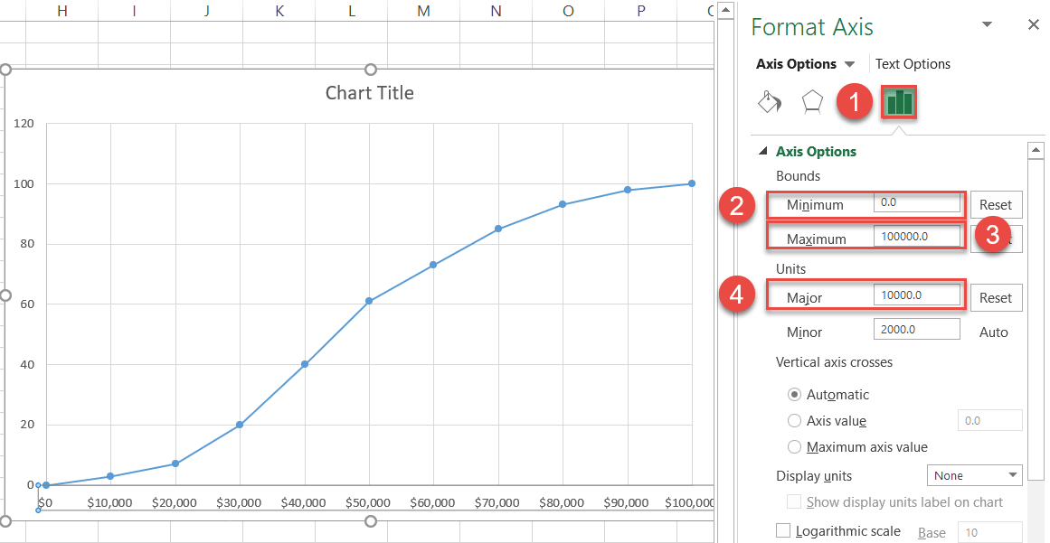
1. Navigate to the Axis Options tab.
2. Set the Minimum Bounds value to the number representing the lowest class limit in the dataset (0).
3. Change the Maximum Bounds value to the number that equals the highest class limit in the dataset (100,000).
4. Set the Major unit value to the class width based on your actual data, the distance between the upper and lower limits of any class in the dataset (10,000).

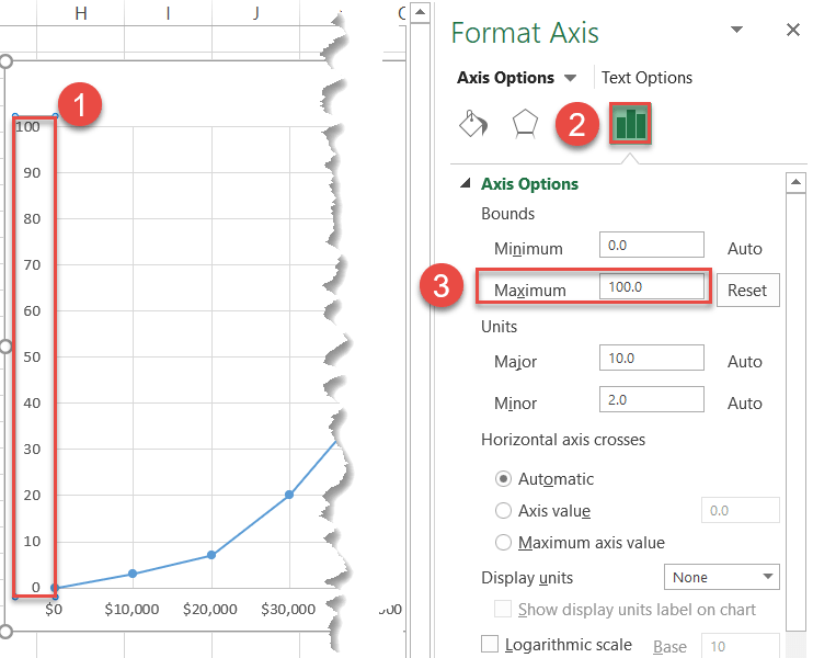
Step #6: Change the vertical axis scale.

Without closing the pane, jump to the vertical axis (the numbers along the left side) and, by the same token, set the Maximum Bounds value to the total amount of the observations (100).

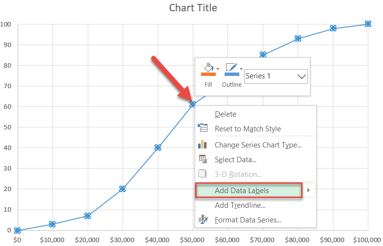
Step #7: Add the data labels.

As we proceed to polish the graph, the next logical step is to add the data labels.

To do that, simply right-click on the chart line and choose “Add Data Labels.”

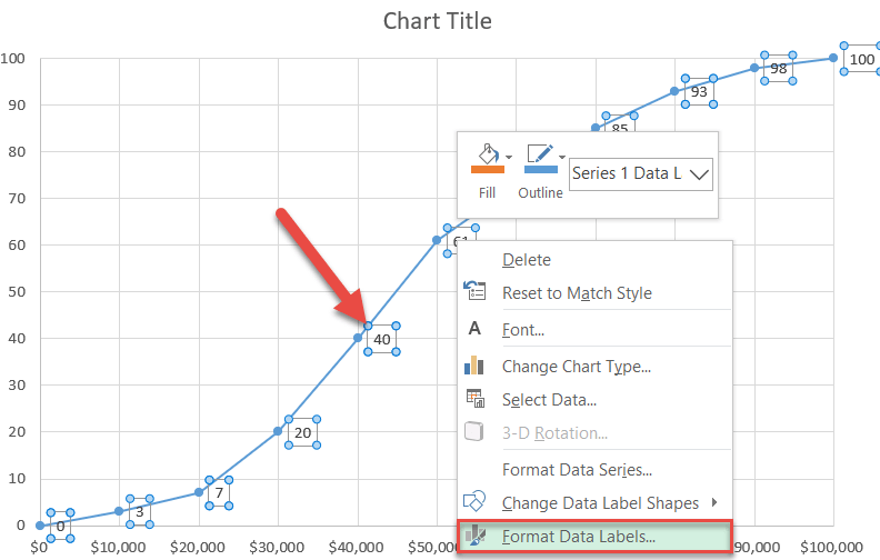
Step #8: Reposition the data labels.

It is important to move the labels up to stop them from overlapping the chart line. Right-click on any data label and select “Format Data Labels.”

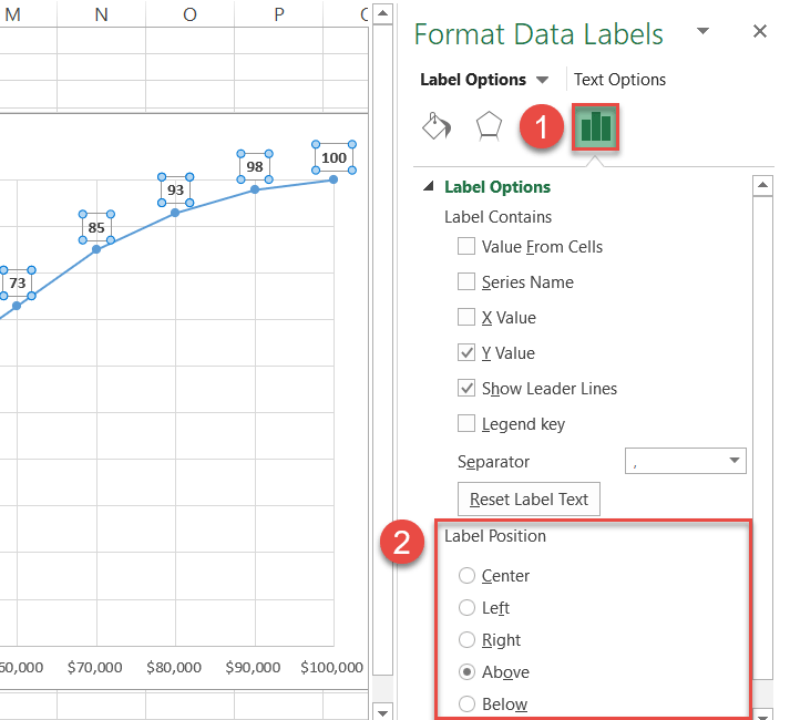
From there, changing label positions is just a couple clicks away:

1. Click the “Label Options” icon.
2. Under Label Position, choose “Above.”

Also, make the labels bold (Home tab > Font) so they stand out.

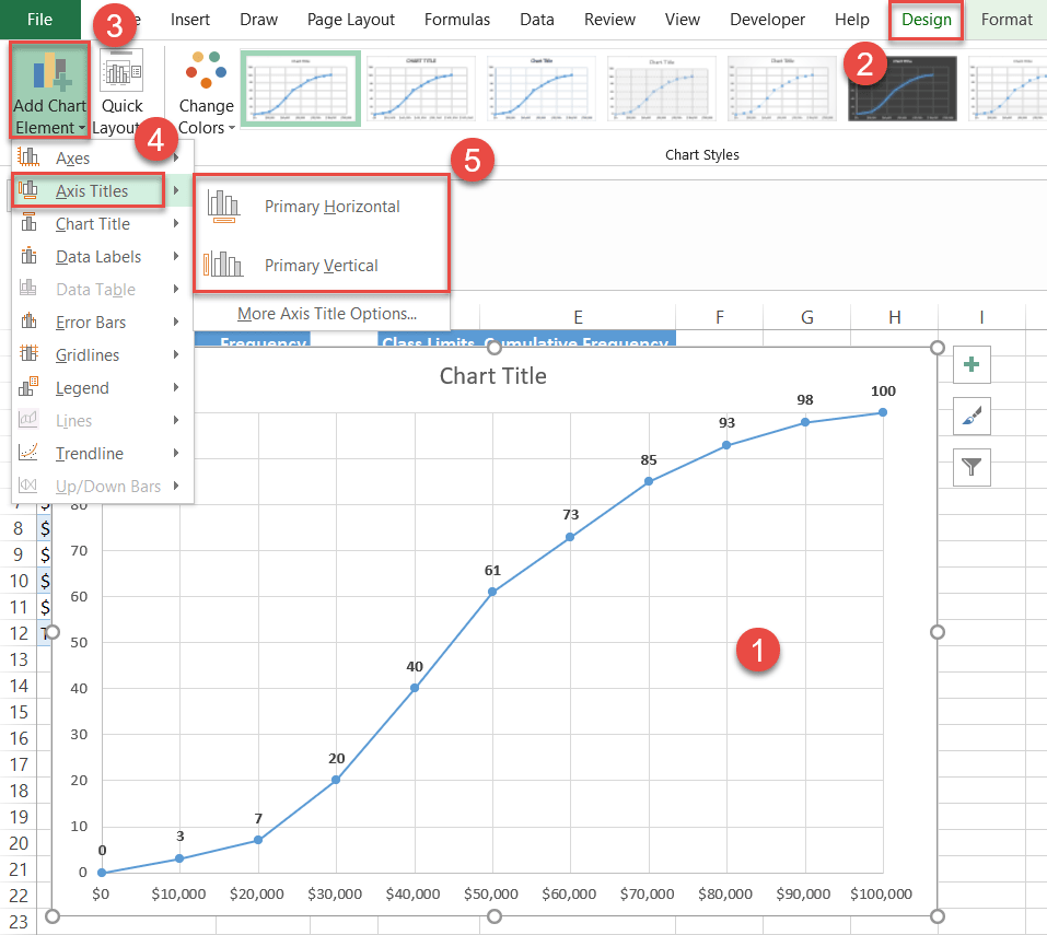
Step #9: Add the axis titles.

Here comes the final step before calling it a day: adding the axis titles.

1. Select the chart plot.
2. Go to the Design tab.
3. Click the “Add Chart Element” button.
4. Choose “Axis Titles.”
5. Pick both “Primary Horizontal” and “Primary Vertical” from the menu that appears.

Rename the chart and axis titles. Don’t forget that you can stretch the chart to make it bigger in order to avoid overlapping data if necessary.

Congratulations on creating your own ogive graph!

You now have all the information you need to create stunning ogive graphs from scratch in Excel to gain a bottomless well of critical data for better decision making.