How to Create a Step Chart in Excel

This tutorial will demonstrate how to create a step chart in all versions of Excel: 2007, 2010, 2013, 2016, and 2019.

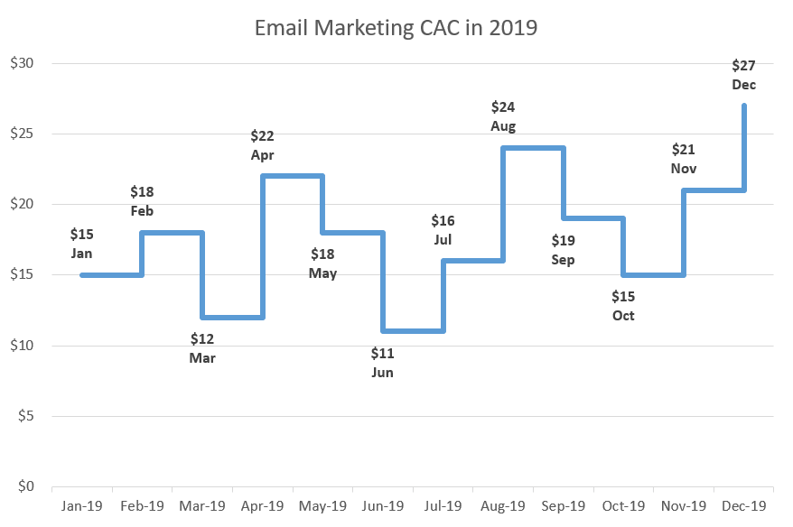
Step charts—which are commonly used to analyze price fluctuations and are cut from the same cloth as line charts—come to the rescue when you need to neatly display regular or sporadic quantitative leaps in values, prices, interest rates, and so forth.

However, since the chart is not supported in Excel, you will have to put in some effort to plot it yourself. To save you time, we developed the Chart Creator Add-in, an easy-to-use tool for creating advanced Excel charts within seconds.

In this step-by-step tutorial, you will learn how to build a simple step chart from scratch in Excel:

Getting Started

For illustration purposes, let’s assume you are about to launch a massive marketing campaign for your brand and need to figure out where to put your ad dollars in 2020.

As you sift through different marketing channels in search of the best-performing option, you set out to plot a step chart displaying your email marketing customer acquisition cost (CAC) from 2019, the pivotal metric that measures the cost of marketing efforts needed to gain a new customer.

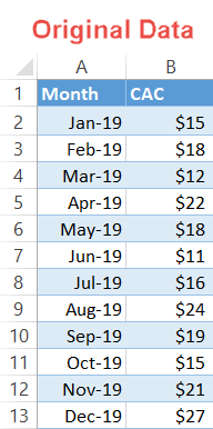
That being said, here is a sample table summarizing the performance of the marketing channel in 2019:

In business, time is money, so let’s get started.

Step #1: Clone the original data table.

Since building a step chart entails a great deal of data manipulation, create a copy of the table containing the original data in order to keep things more organized.

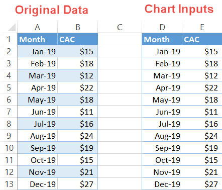
Step #2: Duplicate all the values in the cloned table.

As a workaround for transforming a line chart into a step chart, in the newly-created table, set up two identical sets of data containing the same values.

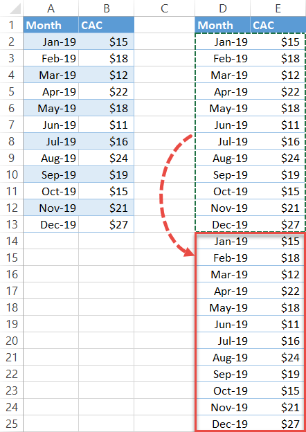
To do that, highlight all the values in the second table and press Ctrl + C to copy the selected cells. Then, select the first empty cell underneath the table (in our case, D14) and press Ctrl + V to paste the data.

Here is how it looks in practice:

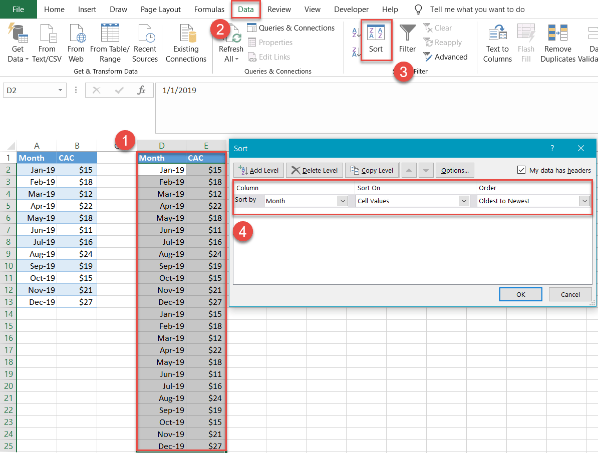
Step #3: Sort the table by the date column from oldest to newest.

It’s time to lay the groundwork for the custom data labels which you will create down the road.

1. Highlight the entire cloned table (D1:E25).
2. Navigate to the Data tab.
3. In the Sort & Filter group, select the “Sort” button.
4. In each dropdown menu, sort by the following:
   1. For “Column,” select “Month” (Column D).
   2. For “Sort On,” select “Values” / “Cell Values.”
   3. For “Order,” select “Oldest to Newest.”
5. Click OK to close the dialog box.

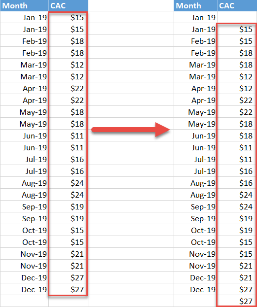
Step #4: Shift the cost values one cell downward.

This simple technique will save you the trouble of having to manually type the values for each date.

Highlight all the values from column CAC (column E) in the duplicate table. Then shift everything one cell downward by pressing Ctrl + X to cut the data then Ctrl + V in the next cell down (E3) to paste it in its new position.

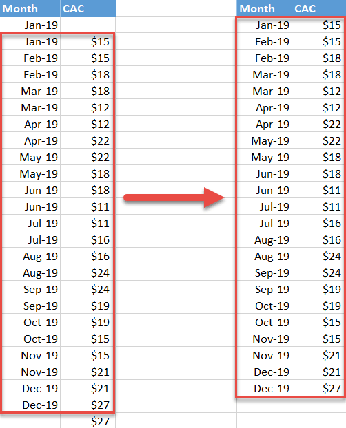
Step #5: Remove the first and last rows of the duplicate table.

Once there, remove the first and last rows of the second table and move the remaining data underneath the column headings so the columns are even again.

Highlight cells D2 and E2, right-click and select Delete. In the dialog box, choose Shift cells up. Do the same for cell E25.

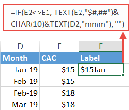
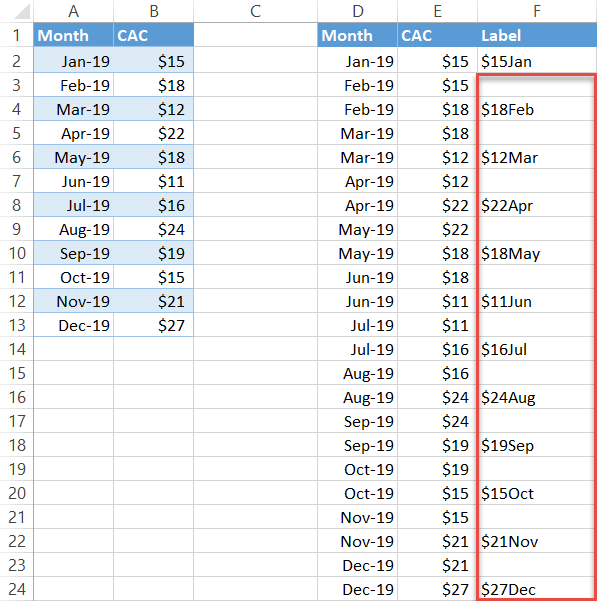
Step #6: Design the custom data labels.

Our next step is designing the custom data labels only for the values in the chart that reflect the original data while leaving out the helper data points, which hold it all together.

First, set up a new data category called “Label” in the column adjacent to the second table (in our case, column F).

Once there, to create the labels containing the dates paired with the corresponding values, you need to unleash the power of IF, CHAR, and TEXT functions. This special cocktail of Excel functions will help us pull off the task:

=IF(E2<>E1, TEXT(E2,"$#,##")&CHAR(10)&TEXT(D2,"mmm"), "")

For the uninitiated, here is the decoded version of the formula:

=IF({The cost in cell E2}<>{The cost in cell E1}, TEXT({The cost in cell E2},"{Format the value as currency }")&CHAR(10)&TEXT({The date in cell D2},"{Format the value in the month format}"), "")

In plain English, the formula compares the values E1 and E2 between themselves, and if they don’t match, cell F2 gets filled with the custom label displaying both the corresponding month and cost. The CHAR(10) function remains a constant and stands for a line break. Otherwise, the formula returns a blank value.

Here is how it looks like when the rubber hits the road:

Now, drag the fill handle in the bottom right corner of the selected cell all the way down to the bottom of column F to execute the formula for the remaining cells (F3:F24).

Step #7: Create a line chart.

All obstacles have now been removed. It’s time to create a simple line chart and see what happens.

1. Highlight all the cells containing the date and cost values (D2:E24).
2. Go to the Insert tab.
3. Click the “Insert Line or Area Chart” icon.
4. Choose “Line.”

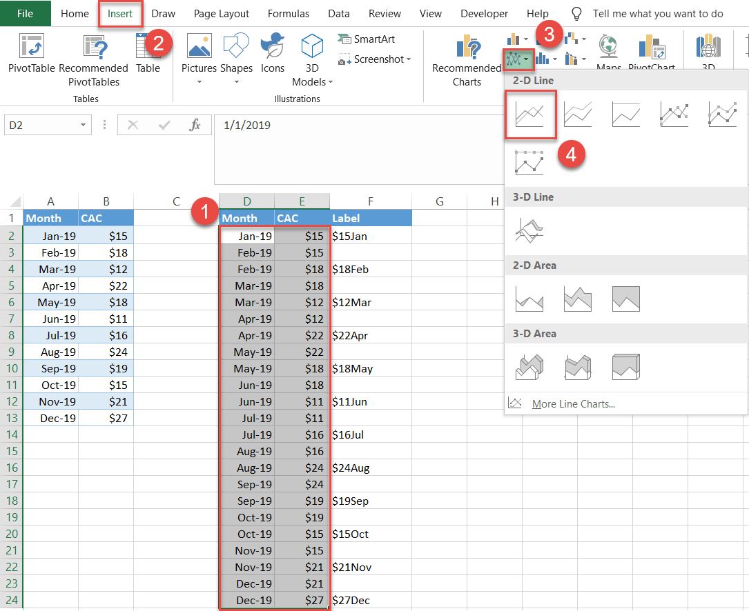
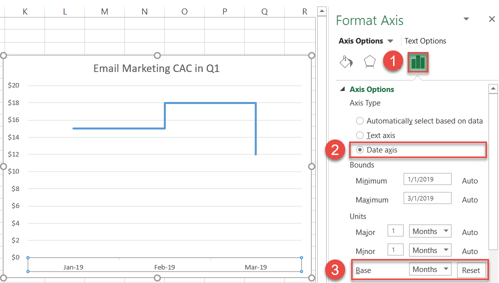
Miraculously, a step chart pops up! However, one caveat is worth mentioning. Suppose you set out to analyze the performance of email marketing only across the span of three months instead:

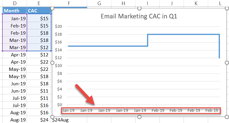
As you may have noticed, the horizontal axis looks quite messy. Fortunately, fixing the issue is as easy as shelling peas. First, right-click on the horizontal axis (the labels along the bottom) and select “Format Axis.”

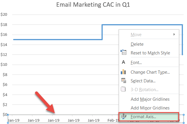
In the task pane that appears, do the following:

1. Switch to the Axis Options tab.
2. Under Axis Type, select the “Date axis” radio button.
3. Under Units, set the Base value to “Days/Month/Year,” depending on your actual data.

Now, back to our step chart.

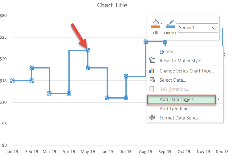
Step #8: Add the data labels.

Next, we need to add to the step chart the custom data labels you have previously crafted.

Right-click on the line illustrating the cost fluctuations and select “Add Data Labels.”

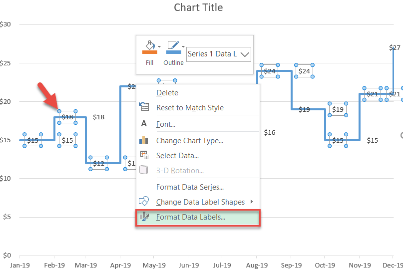
Step #9: Add the custom data labels and get rid of the default label values.

Right-click on any of the labels in the chart and choose “Format Data Labels.”

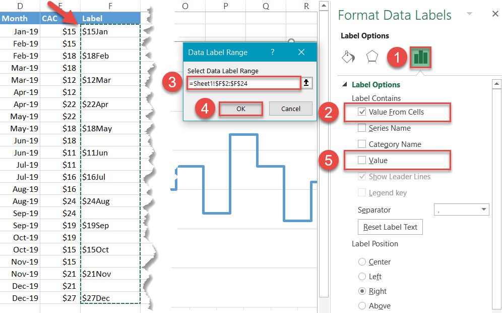
Once the task pane appears, do the following:

1. Go to the Label Options tab.
2. Check the “Value from Cells” box.
3. Highlight all the values from column Label (F2:F24).
4. Click “OK” to close the dialog window.
5. Uncheck the “Value” box to remove the default labels.

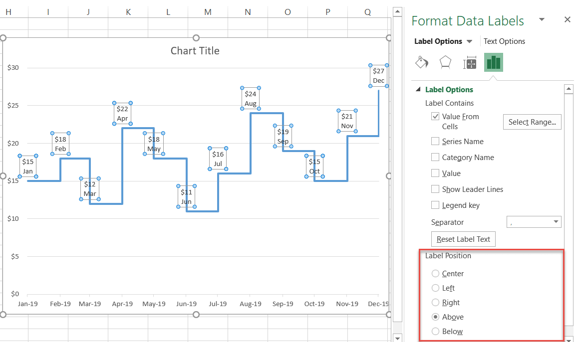
Step #10: Push the labels above the chart line.

We are almost done! As a final touch, you need to get the labels lined up in the right places. The labels representing cost hikes will be placed above the line. Conversely, the labels displaying cost drops will be moved down below the line.

In the Format Data Labels task pane, under the Label Options tab, scroll down to Label Position and select the option “Above.”

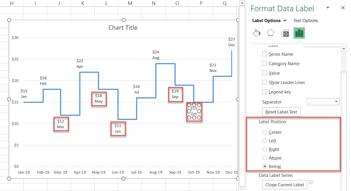
Step #11: Move the labels showing the cost drops down below the chart line.

Finally, select the labels one-by-one that display the drops in the CAC and set the Label Position value for each one to “Below.”

For one last adjustment, make the labels bold (Home tab > Font) and change the chart title. Your step chart is ready.

So there you have it: more information leading to better decisions, all thanks to your step chart!