Conditional Formatting Based on Another Cell – Excel & Google Sheets

This tutorial will demonstrate how to highlight cells based on another cell value using Conditional Formatting in Excel and Google Sheets.

 

 

Highlight Cells Based on Another Cell

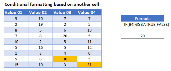
To highlight cells based on another cell’s value, you can create a custom formula within a conditional formatting rule.

1. Select the range you want to apply formatting to.
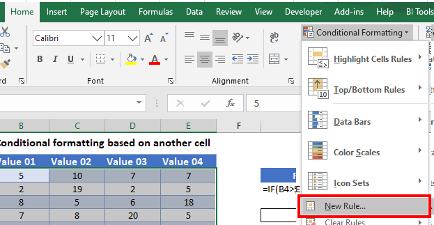
2. In the Ribbon, select Home > Conditional Formatting > New Rule.

 

 

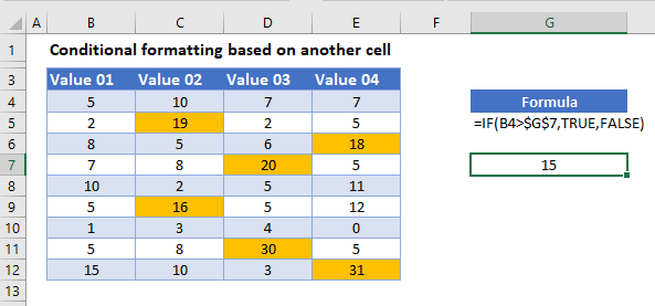
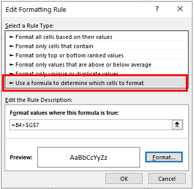
3. Select Use a formula to determine which cells to format, and enter the following formula:

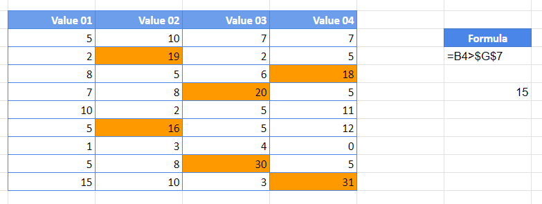
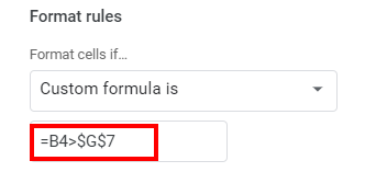
=B4>$G$7

4. Cell G7 needs to be locked by making it an absolute reference. You can do this by using the $ sign around the row and column indicators, or by pressing F4 on the keyboard.
5. Click Format.

 

 

6. Choose the formatting for cells that meet the conditions.

 

 

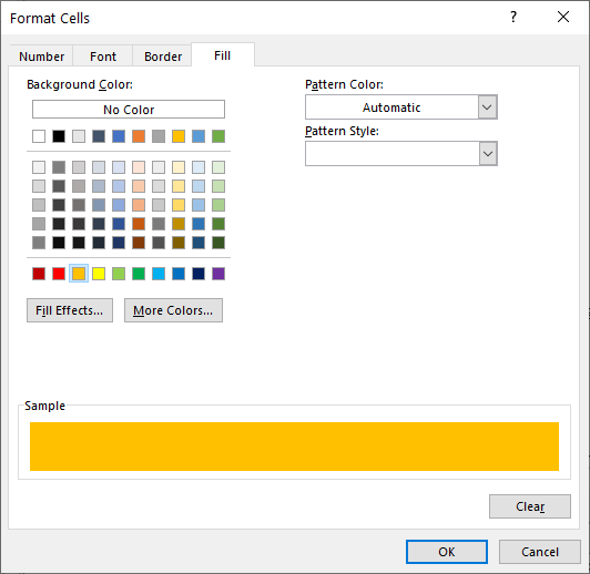
7. Click OK, then OK again to return to the Conditional Formatting Rules Manager.

 

 

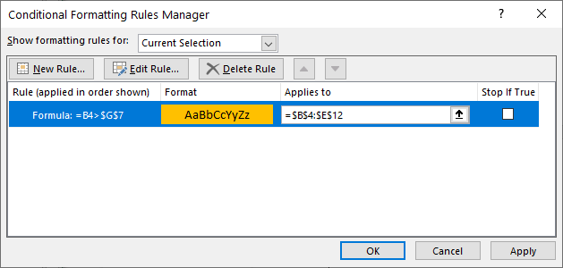
8. Now your range is conditionally formatted if the cell value is greater than the value contained in cell G7.

 

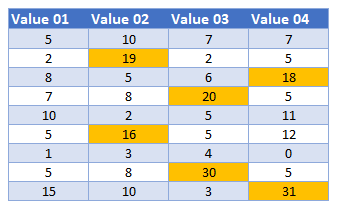
The rule is based on the cell value in G7, so you can then change the value in G7 to see number of formatted cells change!

 

 

Highlight Cells Based on Another Cell in Google Sheets

The process to highlight cells based on another cell in Google Sheets is similar to the process in Excel.

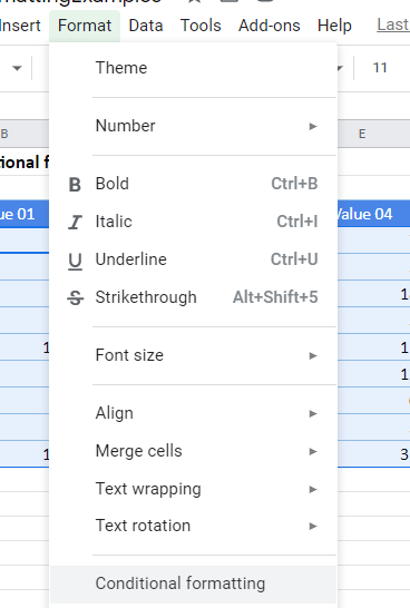
1. Highlight the cells you wish to format, and then click on Format, Conditional Formatting.

 

 

2. The Apply to Range section will already be filled in.

 

 

3. From the Format Rules section, select Custom Formula.

 

 

4. Select the fill style for the cells that meet the criteria.

 

 

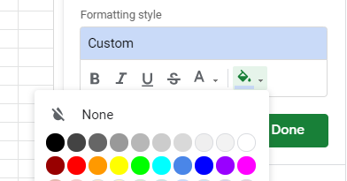
5. Click Done to apply the rule.

 

 

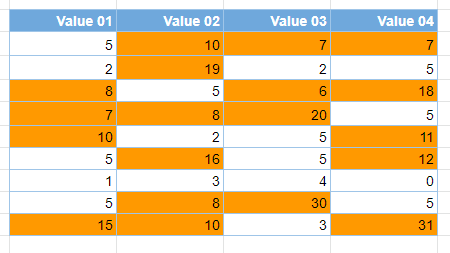
6. Change the value in G7 to see the format of the cells change.