Highlight Blank Cells (Conditional Formatting) – Excel & Google Sheets

This tutorial will demonstrate how to highlight blank cells using Conditional Formatting in Excel and Google Sheets.

 

 

Highlight Blank Cells

To highlight blank cells with Conditional Formatting, use the ISBLANK Function within a conditional formatting rule.

1. Select the range you want to apply formatting to.
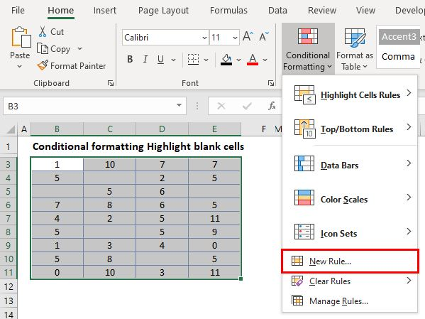
2. In the Ribbon, select Home > Conditional Formatting > New Rule.

 

 

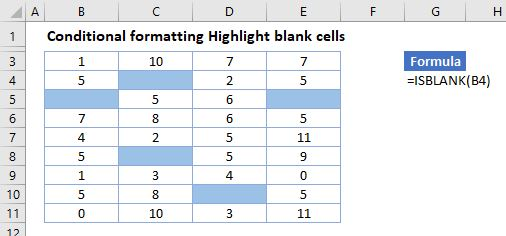
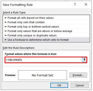
3. Select Use a formula to determine which cells to format, and enter the formula:

=ISBLANK(B3)

 

 

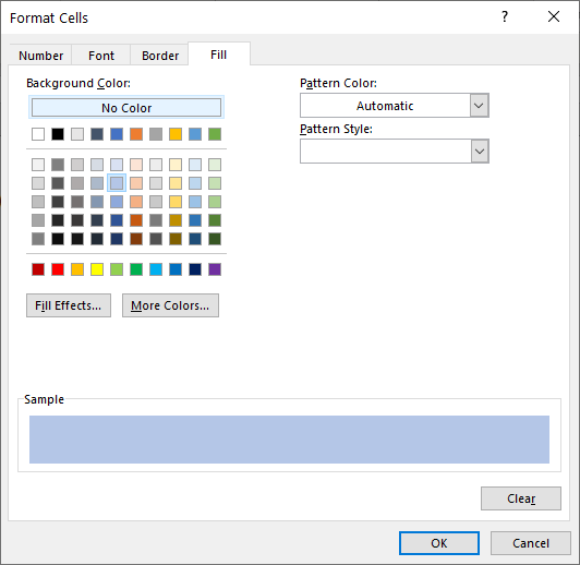
4. Click on the Format button and select your desired formatting.

 

 

5. Click OK, then OK again to return to the Conditional Formatting Rules Manager.

 

 

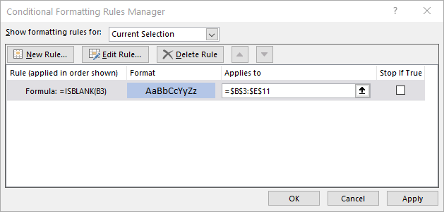
6. Click Apply to apply the formatting to your selected range, then Close.

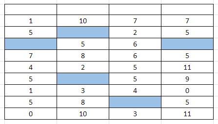
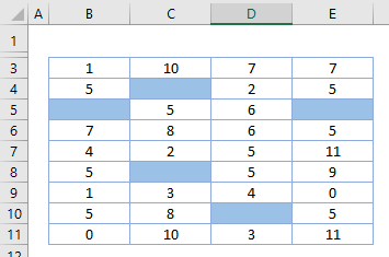
Now blank cells are formatted as specified (blue fill color).

 

 

Highlight Blank Cells – Google Sheets

The process to highlight cells based on the value contained in that cell in Google Sheets is similar to the process in Excel.

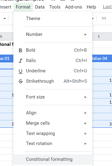
1. Highlight the cells you wish to format, and then click on Format, Conditional Formatting.

 

 

2. The Apply to Range section will already be filled in.

 

 

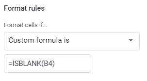
3. From the Format Rules section, select Custom Formula.

 

 

4. Select the fill style for the cells that meet the criteria.

 

 

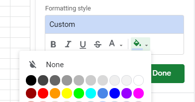
5. Click Done to apply the rule.