Create a Cascading Drop-Down List in Excel & Google Sheets
Written by
Reviewed by
This tutorial will demonstrate how to create a cascading (also called “dependent” or “conditional”) drop-down list in Excel and Google Sheets.
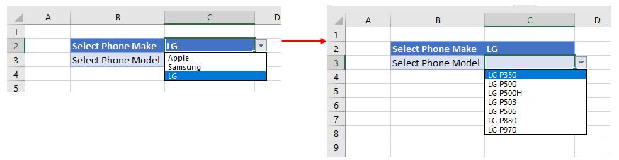
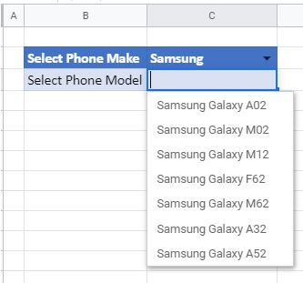
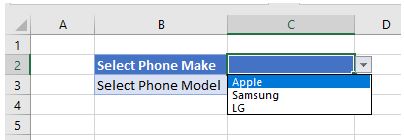
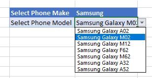
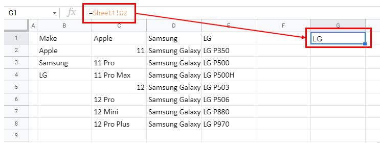
A cascading drop-down list is a list based on the value that is selected in a different list. In the example above, the user has selected LG as the Phone Make. The list showing Phone Models of phones will then show only the LG models. If the user were to select either Apple or Samsung, then the list would change to show the relevant models for those makes of phone.
Create Range Names
The first step in creating cascading drop-down lists is to set a location to store the list data and create range names from those lists of data.
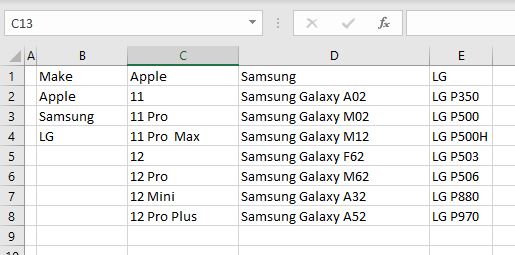
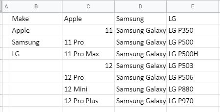
- In a separate location, type in the information that is required for the drop-down lists. This can be in a separate worksheet or in a range of blank cells to the right of the required drop-down lists.
- Then select the data for the first list and create a range name for that data. In the Ribbon, select Formulas > Define Name.
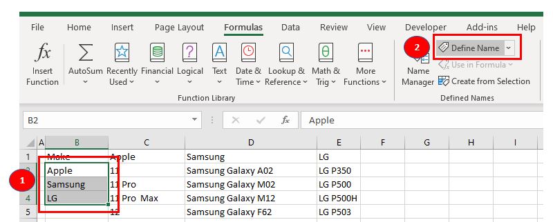
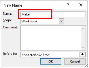
- Type in the name for the range of data, and then click OK.
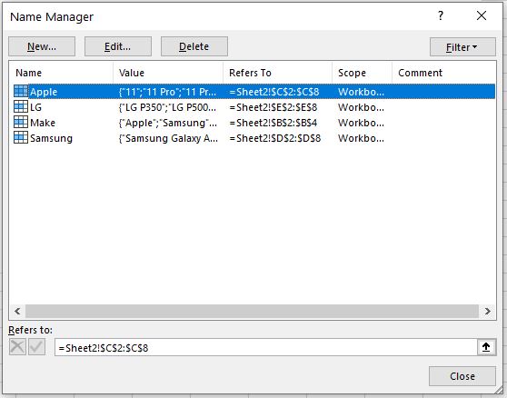
- Repeat this for each of the individual lists (for this example, Apple, Samsung, and LG). After creating the range names, in the Ribbon, select Formulas > Name Manager (or press CTRL + F3 on the keyboard) to see the range names in the Name Manager.
Create the First Drop-Down List Using Data Validation
Drop-down lists are a type of data validation rule.
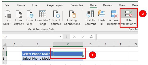
- Select the cell where you want the first (main) drop-down list to go.
- In the Ribbon, select Data > Data Tools > Data Validation.
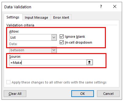
- In the Settings tab, select List under Allow, and ensure that Ignore blank and In-cell dropdown are checked. Type in the name of the range as the Source for the drop-down list.
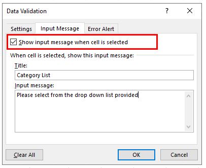
- To set up a message to inform the worksheet users that they need to select from a drop-down list, select the Input Message tab and check the Show input message when cell is selected check box. Type in your Title and input message.
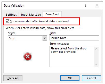
- Select the Error Alert tab and set up a message when the user does not select from the valid drop-down list. Make sure that Show error alert after invalid data is entered is checked, and then select the Style in the drop-down list. Then type in a Title and error message for the warning.
- Click OK to add the data validation rule to the selected cell.
- This will create the first drop-down list showing the different makes of cell phones.
Create Cascading Drop-Down List With Data Validation
- Select the cell where you want the second (dependent) drop-down list to go.
- In the Ribbon, select Data > Data Tools > Data Validation.
- In the Settings tab, select List from the Allow field, and ensure that Ignore blank and In-cell dropdown are checked.
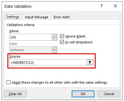
- Type in the following formula and then click OK.
=INDIRECT(C2)Note: You could alternatively use an IF statement.
- If you do not have a value in C2, you will get the error message:
The Source currently evaluates to an error. Do you want to continue?
This is because you have not selected from the drop-down list in C2; click Yes to override the message.
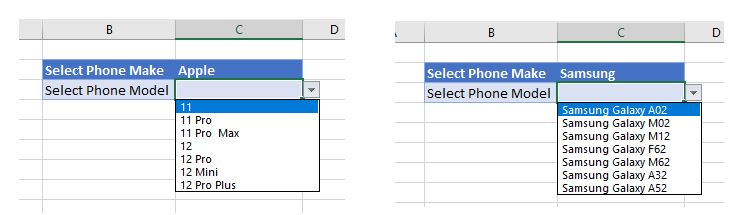
- Select a Phone Make from the first drop-down list, and then select the second drop-down list to see the cascading list.
Create a Cascading Drop-Down list in Google Sheets
Creating a cascading drop-down list in Google Sheets is quite different from creating one in Excel as you cannot use the INDIRECT Function. Instead, use the INDEX and MATCH Functions (which can also be used in Excel).
- As with Excel, the first step in creating cascading drop-down lists is to set a separate location in the sheet to store the list data.
You can then create a named range for the values you want in the first drop-down list.
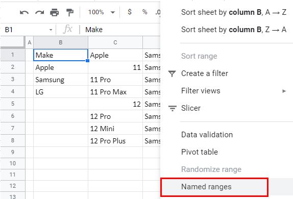
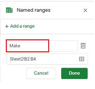
- Select the data for the named range and then from the Menu, select Named ranges.
- Type in the name to give the range, and then click Done.
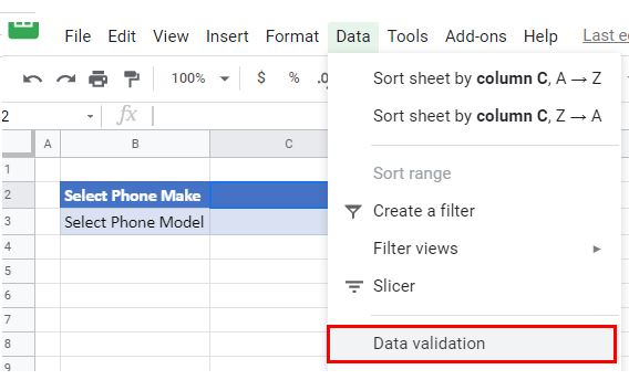
- For the first drop-down list, click in the cell where it needs to appear and then in the Menu, select Data > Data validation.
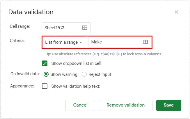
- Set the Criteria by selecting List from a range and typing in the name of the named range you created. Click Save.
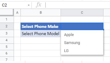
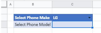
- Select an option from the newly created drop-down list (for example, Apple).
From this point, Google Sheets differs from Excel. Returning to the location where the list data is stored, match the option selected in the first drop-down list with the lists you have created in your data.
- First, create a reference to the selected option.
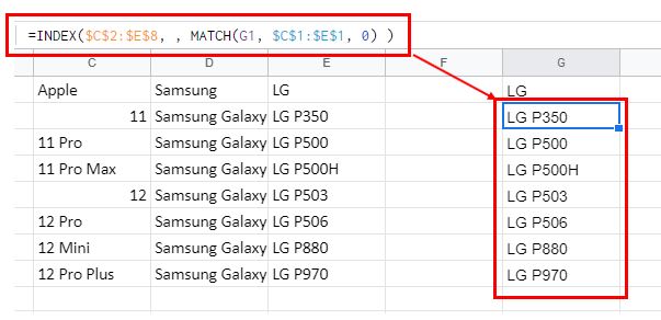
- Then, in the cell beneath the reference, type in the following formula.
=INDEX($C$2:$E$8, , MATCH(G1, $C$1:$E$1, 0) )This formula will look for a matching value in the range C1:E1 (Apple, Samsung, or LG), and return the list directly below that range (C2:E8).
Then use this list as the second range for the cascading drop-down list.
- Select the cell where you want the cascading drop-down list to appear.
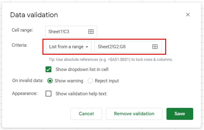
- In the Menu, select Data validation, and then select the range you created above as the range for the list. Click Save.
Now when you change the value of the original drop-down list, the range available in the second drop-down list will also change.