17 Reasons Why Your XLOOKUP is Not Working
This tutorial will demonstrate how to debug XLOOKUP formulas in Excel. If your version of Excel does not support XLOOKUP, read how to use the VLOOKUP instead.
Most errors in our XLOOKUP Formulas are related to XLOOKUP’s properties and criteria. The syntax of the XLOOKUP Function only shows us the necessary arguments to perform the function, but it doesn’t completely inform us about the properties and criteria that are necessary for it to work correctly.
Therefore, in this tutorial, we won’t only learn how to diagnose XLOOKUP errors, but we’ll also understand more about its properties and criteria.
#N/A Error
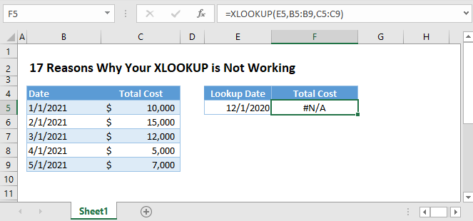
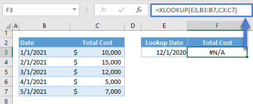
If the XLOOKUP Function fails to find a match, it will return the #N/A Error. Let’s diagnose the problem.
1. #N/A – No Exact Match
By default, the XLOOKUP Function looks for an exact match. If the item is not within the lookup array, then it will return the #N/A Error.
2. #N/A – No Approximate Match
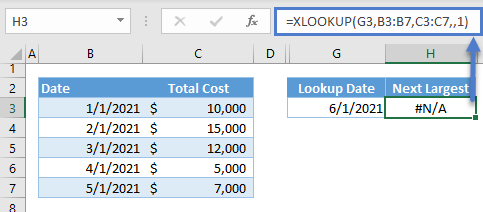
If the match_mode (i.e., 5th argument) is set to -1, the XLOOKUP Function will look for the exact match first, but if there’s no exact match, it will find the largest value from the lookup array that is less than the lookup value. Therefore, if there’s no exact match and all values from the lookup array are greater than the lookup value, the XLOOKUP Function will return the #N/A Error.
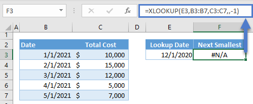
Instead of largest value <= lookup value, we can also look for the opposite, smallest value >= lookup value, if we set the match_mode to 1. The latter condition will find the smallest value that is greater than or equal to the lookup value, and if all values are less than the lookup value, the #N/A Error is returned:
If the value truly does not exist, then the formula is working properly. We recommend adding an error handling so that if the value is not found, a different value is outputted instead of the #N/A error:
=XLOOKUP(G3,B3:B7,C3:C7,"No match!",1)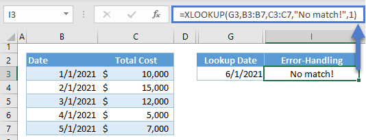
However, if the lookup value exists and the XLOOKUP Function can’t find it, here are some possible reasons:
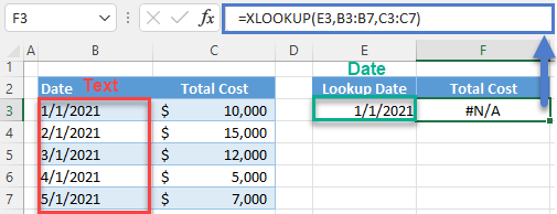
3. #N/A – Numbers Stored as Text (and Other Data-type Mismatches)
One of the important criteria of XLOOKUP is that the data types of the lookup value and lookup array must be the same. If not, the XLOOKUP Function won’t be able to find a match.
The most common example of this is numbers stored as text.
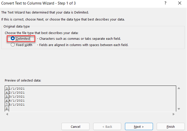
One way to solve this is to use the Text to Columns Tool of Excel to convert numbers stored as text into numbers.
Here are the steps:
- Highlight the cells and go to Data > Data Tools > Text to Columns
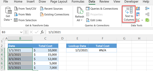
- In the popup window, select Delimited and click Next.
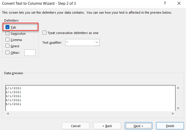
- In the next step, select Tab and click Next.
- In the last step, select the required data type (e.g., date) and the format and click Finish.
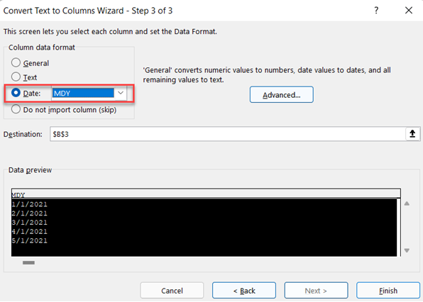
- The range will be converted into the set data type (e.g., date)
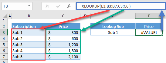
4. #N/A – Extra Spaces
Text lookups are prone to errors due to extra spaces. In this example, the lookup value, “Sub 2,” contains two spaces, and therefore, it won’t match with “Sub 2” (one space) from the lookup array.
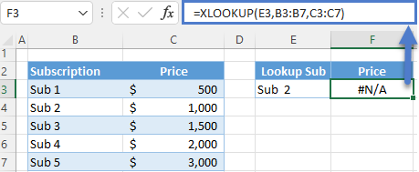
One way to solve this is by using the TRIM Function to remove the extra spaces. We can apply it to both the lookup value and the whole lookup array.
=XLOOKUP(TRIM(E3),TRIM(B3:B7),C3:C7)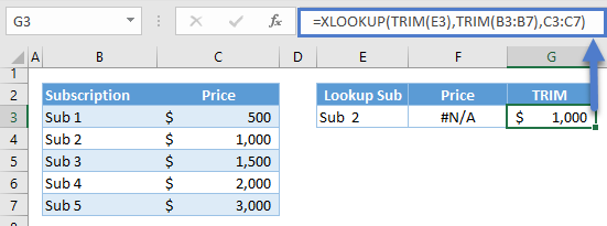
Note: The TRIM Function removes extra spaces between words until there’s a one space boundary between them, and any spaces before the first word and after the last word of a text or phrase are removed.
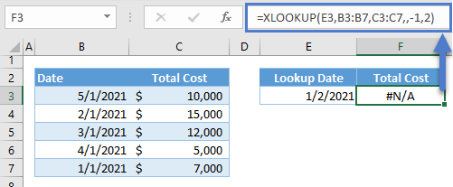
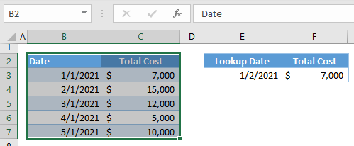
5. #N/A – Lookup Array Not Sorted
If the 6th argument (i.e., Search_Mode) of the XLOOKUP Function is set to either 2 or -2, the XLOOKUP Function will use the binary search method to look up the value, and this method requires a sorted data set (i.e., 2 – ascending order, -2 – descending order). If the lookup array is not sorted, the XLOOKUP Function will return either a wrong value or the #N/A Error:
To solve the above problem, we need to sort the data either manually or through formulas:
Sort Manually
- Highlight the whole data, and then go to Data Tab > Sort & Filter > Click Sort.
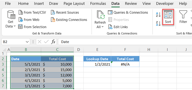
- A pop-up window will appear. Select the column of the lookup array and set the order to the required order (e.g., ascending or oldest to newest for dates). Click OK.
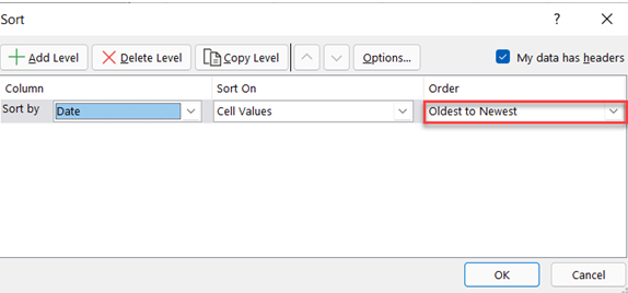
- The data will be sorted based on the lookup array (e.g., B3:B7). The XLOOKUP is now recalculated and shows the correct result.
Sort using the SORT Function and SORTBY Function
We can also use the SORT Function and SORTBY Function to sort the lookup array (e.g., B3:B7) and return array (e.g., C3:C7), respectively.
=XLOOKUP(E3,SORT(B3:B7),SORTBY(C3:C7,B3:B7),,-1,2)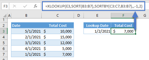
Note: By default, both SORT and SORTBY functions sort an array in ascending order. The main difference between the two is that the SORT Function will always return all columns within an array while the SORTBY Function can return a specific column (e.g., C3:C7) from an array.
#VALUE! Error
If an input doesn’t satisfy the criteria for performing XLOOKUP, the function won’t work and will instead return the #VALUE! Error.
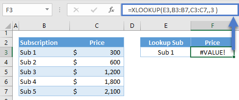
6. #VALUE! – Non-Uniform Row Sizes
A requirement of the XLOOKUP Function (for a typical vertical lookup) is that the row sizes of the lookup array and the return array must be the same.
7. #VALUE! – Horizontal vs. Vertical
The return array can be 2-dimensional and return multiple columns (or rows for a horizontal lookup). However, the number of rows (or columns) must match.
This property enables the XLOOKUP Function to return more than one column (or row for a horizontal lookup), but the consequence is that we can’t pair a 1D horizontal return array to a 1D vertical lookup array unlike the INDEX-MATCH Formula where we can do opposite orientations:
=INDEX(E2:I2,MATCH(D5,B3:B7,0))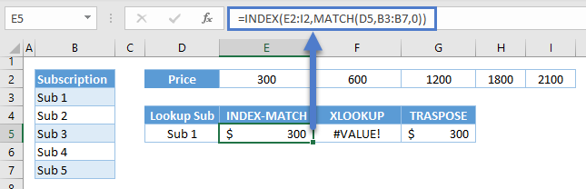
If you do this, the XLOOKUP will accept the return array as a 2D input with a row size not matching the row size of the lookup array. Therefore, it returns the #VALUE! Error.
=XLOOKUP(D5,B3:B7,E2:I2)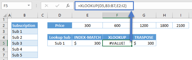
To solve this, we can use the TRANSPOSE Function to transpose the orientation of one of the 1D arrays:
=XLOOKUP(D5,B3:B7,TRANSPOSE(E2:I2))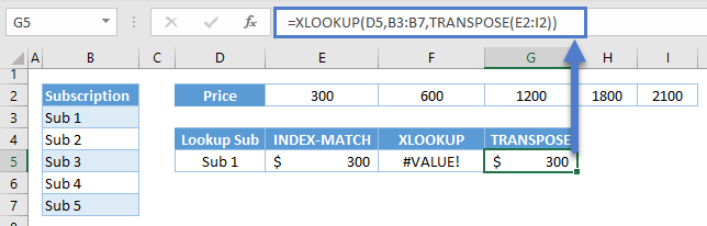
Note: The TRANSPOSE Function switches the relative row and column coordinates of a cell in a list. In E2:I2, F2 is row 1, column 2 relative to the range. Therefore, the transposed coordinates will be row 2, column 1. G2 is row 1, column 3 and is transposed to row 3, column 1 and so on.
8. #VALUE – Value Range
The 5th (match mode) and 6th (search mode) arguments of the XLOOKUP Function must have valid inputs. If not, then the XLOOKUP will return the #VALUE! Error.
Note: The match_mode can only accept 0, -1,1 and 2 while the search_mode can only accept 1,-1,2 and-2.
#NAME? Error
The #NAME? Error is triggered by:
- Misspelling the function’s name
- Misspelling a reference (workbook/sheet reference and named ranges).
- A non-existent Named Range
- Text not enclosed with double quotation marks.
9. #NAME? – Function Name Typo
If there’s a typo in a function’s name, Excel will return the #NAME? Error.
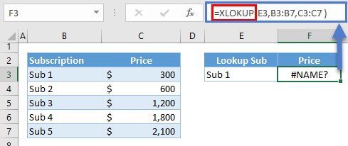
10. #NAME? – Named Range doesn’t Exist
The #NAME? Error can also be caused by an undefined named range in the formula. It’s either the named range doesn’t really exist or there’s a typo in the name.
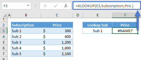
Note: There are two named ranges in the above sheet: Subscription and Price. The typo in the Price named range results to a named range that doesn’t exist, and any text that is not enclosed with quotation marks is considered as a named range, which can also lead to the #NAME? Error.
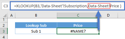
11. #NAME? – Workbook/Sheet Reference Typo
When workbook/sheet names contain spaces and special characters except for underscore, we need to enclose the workbook/sheet reference with single quotations. If this is not satisfied, then Excel can’t recognize the workbook/sheet reference and will return the #NAME? Error.
#SPILL! ERROR
There’s also a set of criteria when returning an array output, and if those criteria are not satisfied, the SPILL! Error is returned instead of the array output.
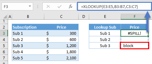
12. #SPILL! – Spill Block
A dynamic array formula will not overwrite the values that are within its spill range. Instead, the array output will be blocked, and the #SPILL! Error is returned.
13. #SPILL! – Table vs. Dynamic Arrays
We can’t use Array XLOOKUP Formulas in Tables because they don’t support dynamic array formulas.
Instead you must use a non-array XLOOKUP Function where the lookup_value is a single value, not an array of values.
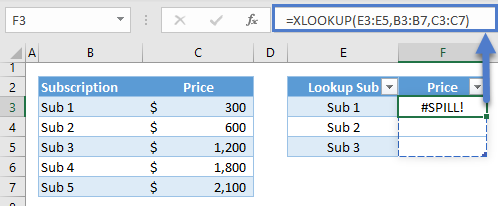
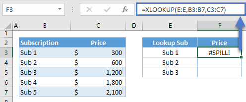
14. #SPILL! – Range Out of Bounds
If the size of the output array from an XLOOKUP formula exceeds the sheet boundaries (row and column), the #SPILL! Is returned instead. (e.g, F3:F < whole column array)
Other Problems
There are XLOOKUP problems that don’t trigger errors because they don’t violate any of the criteria.
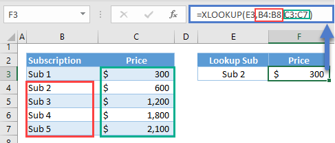
15. Incorrect Range
Even if the row sizes of the lookup array and return array are the same, if their positions do not match with each other, the XLOOKUP will return an incorrect result.
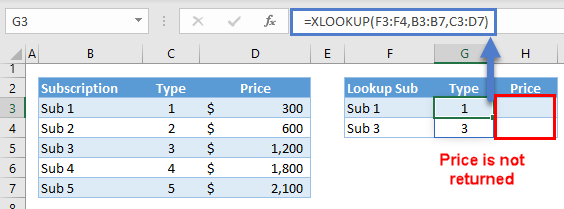
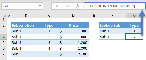
16. 1D/2D Array of Lookup Values vs. 2D Return Array
The lookup value in XLOOKUP can be a 1D or 2D array, which converts the XLOOKUP Function into a dynamic array that will Spill into adjacent cells.
We might expect that a combination of a 1D lookup value array (e.g., F3:F4) and a 2D return array (e.g., C3:D7) will return a 2D output where the row size and column size are dependent on the lookup value array and 2D return array, respectively, but this is not the case. The row size will still be based on the 1D lookup value array, but the column size will be 1, which means that only the 1st column of the return array will be returned.
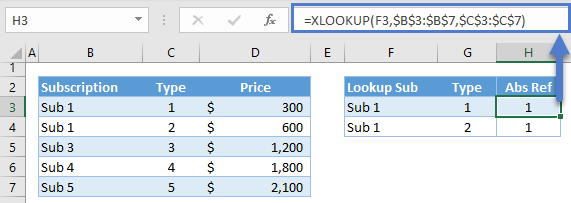
17. Copying XLOOKUP with Relative References
If we drag an XLOOKUP Formula with relative references, then the references will also adjust relative to their position from the reference formula, which can lead to incorrect results.
If we want to copy or drag our XLOOKUP Formula to succeeding cells, we must convert the references for the lookup array and return array to absolute references. We can do this by adding the dollar symbol at the front of the column letter and row number or by pressing F4 while the cursor is in the reference within the formula.