XLOOKUP with IF
This tutorial will demonstrate how to combine the XLOOKUP and IF functions in Excel. If your version of Excel does not support XLOOKUP, read how to use VLOOKUP instead.
XLOOKUP Multiple Lookup Criteria
There are a lot of ways to use the IF Function alongside the XLOOKUP Function, but first, let’s look at an example using the core element of the IF Function, the logical criteria.
One common example is performing a lookup with multiple criteria, and the most common solution to this is by concatenating the lookup criteria (e.g., F3&G3) and their corresponding column in the lookup data (e.g., B3:B7&C3:C7).
=XLOOKUP(F3&G3,B3:B7&C3:C7,D3:D7)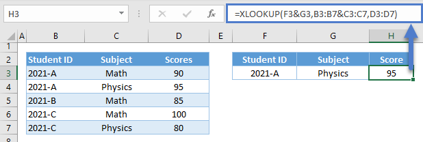
The above method works fine most of the time, but it can lead to incorrect results for conditions that involve numbers.
A more foolproof method is by creating an array of Boolean values from logical criteria.
=XLOOKUP(1,(B3:B7=F3)*(C3:C7=G3),D3:D7)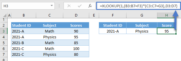
Let’s walk through this formula:
Logical Criteria
First, let’s apply the appropriate condition to their corresponding columns by using the logical operators (e.g., =,<,>).
Let’s start with the first criterion (e.g., Student ID).
=B3=$C$2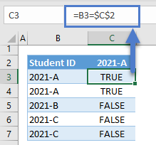
Repeat the step for the other criteria (e.g., Subject).
=D3=$E$2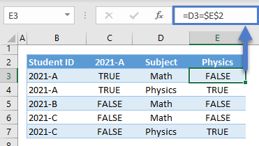
Array AND
Next, we perform the array equivalent of the AND Function by multiplying the Boolean arrays where TRUE is 1 and FALSE is 0.
=C3*E3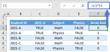
Note: The AND Function is an aggregate function (many inputs to one output). Therefore, it won’t work in our array scenario.
XLOOKUP Function
Next, we use the result of the Array AND as the new lookup array where we will lookup for 1 instead of the original lookup value.
=XLOOKUP(1,F3:F7,G3:G7)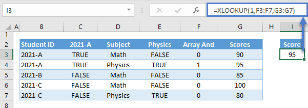
Combining all formulas above results to our original formula:
=XLOOKUP(1,(B3:B7=F3)*(C3:C7=G3),D3:D7)
XLOOKUP Error-Handling with IF
Sometimes we need to check if the result of an XLOOKUP Function results in an error. A great way of doing this is by using the IF Function, which is also the best way of notifying us about the cause of the error.
XLOOKUP IF with ISNA
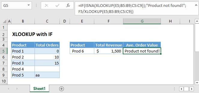
Let’s first check if the XLOOKUP failed to find a match using the IF with ISNA Formula.
=IF(ISNA(XLOOKUP(E3,B3:B7,C3:C7)),"Product not found!",F3/XLOOKUP(E3,B3:B7,C3:C7))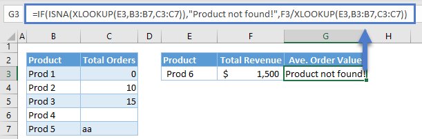
Let’s walk through the above formula:
ISNA Function
First, let’s check for the #N/A Error, which basically means no match was found, using the ISNA Function.
=ISNA(XLOOKUP(E3,B3:B7,C3:C7))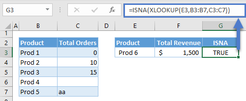
IF Function
Next, let’s use the IF Function to check the result of the ISNA Function and return a message (e.g., “Product not found!”) if the result is TRUE. Otherwise, if the result is false, we’ll proceed with the calculation.
=IF(G3,"Product not found!",F3/XLOOKUP(E3,B3:B7,C3:C7))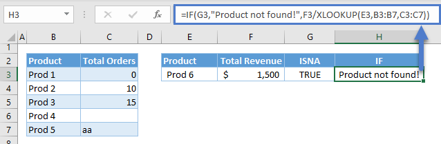
Combining all formulas results to our original formula:
=IF(ISNA(XLOOKUP(E3,B3:B7,C3:C7)),"Product not found!",F3/XLOOKUP(E3,B3:B7,C3:C7))
XLOOKUP IF with ISBLANK
Another thing to check is if the result of XLOOKUP is blank. There are cases where blank means there’s no input yet, and therefore, we need to distinguish it from zero.
We’ll just replace the ISNA with ISBLANK to check for blank.
=IF(ISBLANK(XLOOKUP(E3,B3:B7,C3:C7)),"No data!",F3/XLOOKUP(E3,B3:B7,C3:C7))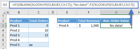
Let’s walk through the above formula:
ISBLANK Function
First, let’s check for blank using the ISBLANK Function.
=ISBLANK(XLOOKUP(E3,B3:B7,C3:C7))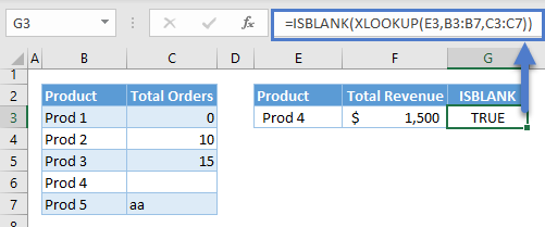
IF Function
Just like with the previous scenario, we then input the result of the ISBLANK Function to the IF Function and return a message (e.g., “No Data!”) if TRUE or proceed with the calculation if FALSE.
=IF(G3,"No data!",F3/XLOOKUP(E3,B3:B7,C3:C7))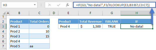
Combining all formulas results to our original formula:
=IF(ISBLANK(XLOOKUP(E3,B3:B7,C3:C7)),"No data!",F3/XLOOKUP(E3,B3:B7,C3:C7))
XLOOKUP IF with ISTEXT
Another thing to avoid in calculations is accidental text input. In this case, we’ll use the IF with ISTEXT Formula to check for a text value.
=IF(ISTEXT(XLOOKUP(E3,B3:B7,C3:C7)),"Invalid input!",F3/XLOOKUP(E3,B3:B7,C3:C7))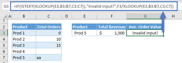
ISTEXT Function
First, we check if the output of the XLOOKUP Function is a text.
=ISTEXT(XLOOKUP(E3,B3:B7,C3:C7))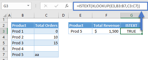
IF Function
Next, we check the result using the IF Function and return the corresponding message (e.g., “Invalid input!”) if TRUE or proceed to the calculation if FALSE.
=IF(G3,"Invalid input!",F3/XLOOKUP(E3,B3:B7,C3:C7))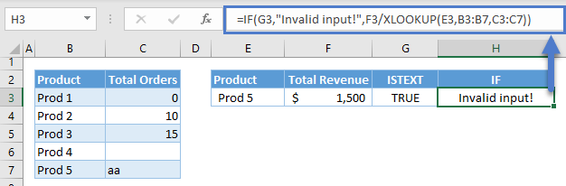
XLOOKUP with IFS
The final error-handling formula would be the combination of the previous IF Formulas, and we can do this by nesting them.
=IF(ISNA(XLOOKUP(E3,B3:B7,C3:C7)),"Product not found!",
   IF(ISBLANK(XLOOKUP(E3,B3:B7,C3:C7)),"No data!",
     IF(ISTEXT(XLOOKUP(E3,B3:B7,C3:C7)),"Invalid input!",F3/XLOOKUP(E3,B3:B7,C3:C7))
   )
 )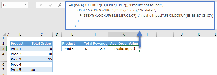
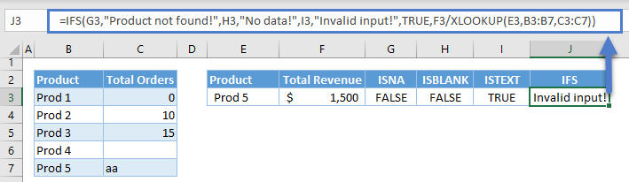
As we notice above, the Nested IF Formula becomes more complicated as we add more conditions. A better way to approach this is by using the IFS Function.
=IFS(ISNA(XLOOKUP(E3,B3:B7,C3:C7)),"Product not found!",
         ISBLANK(XLOOKUP(E3,B3:B7,C3:C7)),"No data!",
         ISTEXT(XLOOKUP(E3,B3:B7,C3:C7)),"Invalid input!",
         TRUE,F3/XLOOKUP(E3,B3:B7,C3:C7)
         )
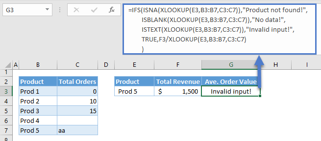
Note: The IFS Function can evaluate multiple sets of logical criteria. It starts from the first condition moving on to the next until it finds the first TRUE condition and returns the corresponding return value to it.
Let’s walk through the formula above:
ISNA
We start with our first condition, which is the ISNA Function. If ISNA is TRUE, we return its corresponding value (e.g., “Product not found!”). Otherwise, we proceed to check the next condition.
=ISNA(XLOOKUP(E3,B3:B7,C3:C7))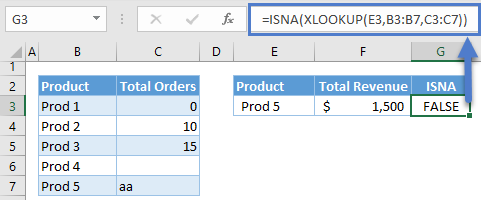
ISBLANK and ISTEXT
Since the first condition is FALSE in this scenario, we check the succeeding conditions until we find the first TRUE and return the corresponding value for the TRUE condition.
=ISBLANK(XLOOKUP(E3,B3:B7,C3:C7))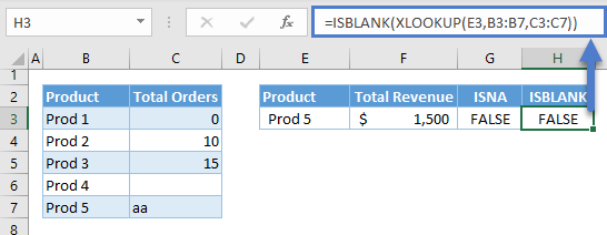
=ISTEXT(XLOOKUP(E3,B3:B7,C3:C7))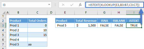
Default Value
We can set a default value by setting the last condition as TRUE in case all the conditions are FALSE, which in our error-handling scenario, means that we can now proceed to the calculation without errors.
Combining all formulas above results to our original formula:
=IFS(ISNA(XLOOKUP(E3,B3:B7,C3:C7)),"Product not found!",
         ISBLANK(XLOOKUP(E3,B3:B7,C3:C7)),"No data!",
         ISTEXT(XLOOKUP(E3,B3:B7,C3:C7)),"Invalid input!",
         TRUE,F3/XLOOKUP(E3,B3:B7,C3:C7)
         )

