Double (Nested) XLOOKUP – Dynamic Columns – Excel

This tutorial will demonstrate how to perform a Double (Nested) XLOOKUP in Excel. If you don’t have access to XLOOKUP, instead you can perform a nested VLOOKUP.

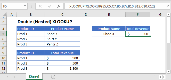
In scenarios where one criterion of a lookup task is dependent on another lookup, we can use the Double (Nested) XLOOKUP to perform the nested lookups.

There are at least three arguments in XLOOKUP where we can input another XLOOKUP: the lookup value (1^st argument), lookup array (2^nd argument) and return array (3^rd argument).

Let’s explore each of the cases.

 

XLOOKUP in Lookup Value

We can nest a XLOOKUP into the lookup_value of another XLOOKUP.

=XLOOKUP(XLOOKUP(E3,C3:C5,B3:B5),B8:B10,C8:C10)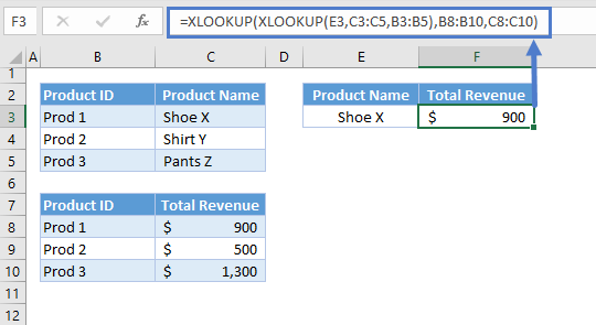

You would do this when the lookup_value (e.g., Product ID) is dependent on another value (e.g., Product name).

Let’s walkthrough the formula:

First, we need to extract the required lookup value for the main XLOOKUP:

=XLOOKUP(E3,C3:C5,B3:B5)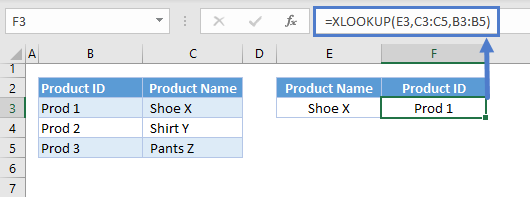

 

The result of the 1^st XLOOKUP is then fed to the main XLOOKUP to perform a lookup at the 2^nd table:

=XLOOKUP(F3,B8:B10,C8:C10)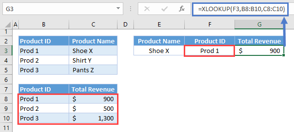

Combining these two lookup processes results to our original formula:

=XLOOKUP(XLOOKUP(E3,C3:C5,B3:B5),B8:B10,C8:C10)

 

XLOOKUP in Lookup Array

Alternatively, we can use a nested XLOOKUP to return the lookup_array.

=XLOOKUP(G3,XLOOKUP(F3,B2:C2,B3:C5),D3:D5)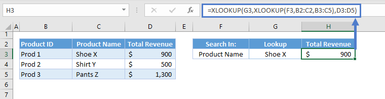

One important property of the XLOOKUP Function is that it can return a 1D array (vertical or horizontal) if the given return array is in 2D (i.e., table). In this case, If the lookup array is a vertical list, then the XLOOKUP Function will return a row, and if the lookup array is a horizontal list, it will return a column.

Let’s breakdown and visualize the formula:

First, we need to perform a lookup in the headers (e.g., column (or row) headers) and return the corresponding column (or row):

=XLOOKUP(G3,B2:C2,B3:C5)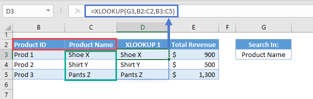

Since the return array is 2D (e.g., B3:C5) and the lookup array is a horizontal list (e.g., B2:C2), the XLOOKUP will return a row (e.g., C3:C5).

The output array from this XLOOKUP is then fed to the lookup array of our main XLOOKUP:

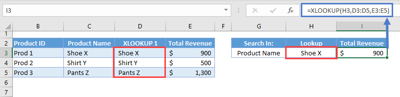
Putting all of these together results to our original formula:

=XLOOKUP(G3,XLOOKUP(F3,B2:C2,B3:C5),D3:D5)

 

XLOOKUP in Return Array

Similarly, we can use a nested XLOOKUP to return a dynamic return_array.

=XLOOKUP(G3,B3:B5,XLOOKUP(H3,C2:E2,C3:E5))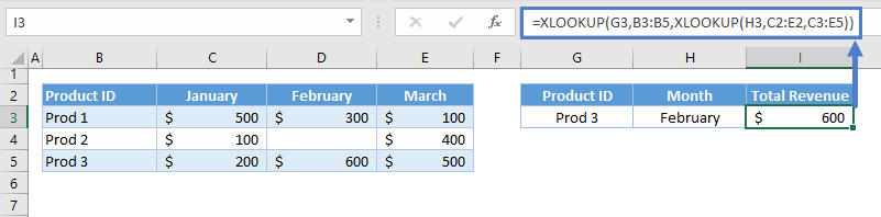

 

Let’s breakdown and visualize the formula:

We use the column headers as the lookup array for the first XLOOKUP:

=XLOOKUP(G3,C2:E2,C3:E5)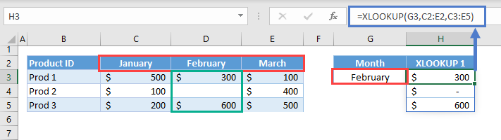

Just like in the previous section, the XLOOKUP will return a row once it finds a match from the column headers.

The resulting output array is used as the return array of our main XLOOKUP:

=XLOOKUP(I3,B3:B5,H3:H5)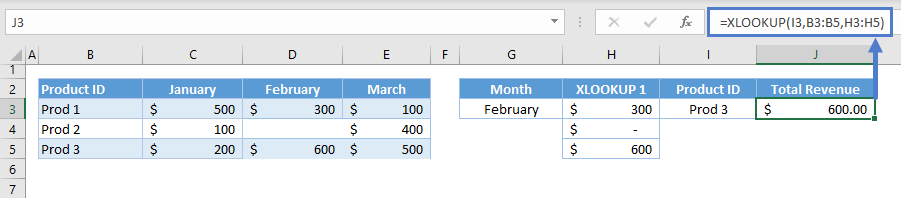

 

Combining these two results to our original formula:

=XLOOKUP(G3,B3:B5,XLOOKUP(H3,C2:E2,C3:E5))