Nested VLOOKUP – Excel & Google Sheets
Written by
Reviewed by
Download the example workbook
This tutorial will demonstrate how to perform a Nested VLOOKUP in Excel and Google Sheets. If you have access to the XLOOKUP Function, we recommend performing a nested XLOOKUP instead.
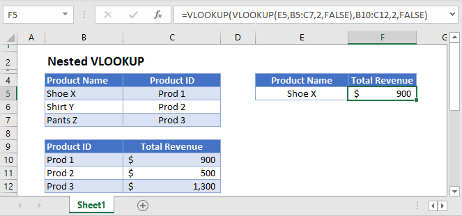
If you need to perform a lookup that is dependent on looking up another value, you can use a Nested VLOOKUP formula:
=VLOOKUP(VLOOKUP(E3,B3:C5,2,FALSE),B8:C10,2,FALSE)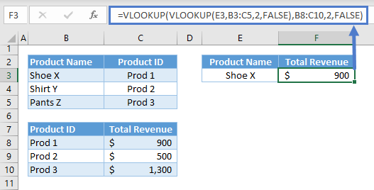
Let’s walkthrough the formula:
First, we need to perform the 1st VLOOKUP to extract the required lookup value (e.g., Product ID) for our main VLOOKUP:
=VLOOKUP(E3,B3:C5,2,FALSE)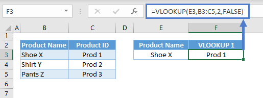
Note: The VLOOKUP Function performs a vertical lookup in the first column of the table array starting from the top of the list going down (i.e., top-down). If it finds a match, it returns the corresponding value from the column described by the column index, and if not, it returns an error.
Next, we substitute the result to our main VLOOKUP and perform a lookup in another table:
=VLOOKUP(F3,B8:C10,2,FALSE)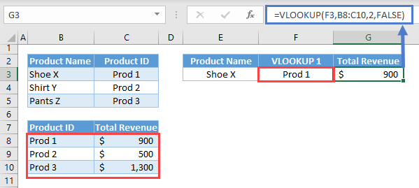
Combining all of these results to our original formula:
=VLOOKUP(VLOOKUP(E3,B3:C5,2,FALSE),B8:C10,2,FALSE)
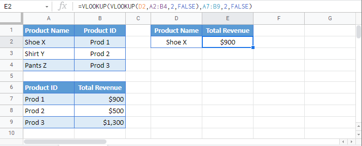
Nested VLOOKUP in Google Sheets
The formula works the same way in Google Sheets: