INDEX MATCH – Excel & Google Sheets

This tutorial will teach you how to use the INDEX & MATCH combination to perform lookups in Excel and Google Sheets.

INDEX & MATCH, The Perfect Pair

Let’s take a closer look at some of the ways you can combine the INDEX and MATCH functions. The MATCH function is designed to return the relative position of an item within an array, while the INDEX function can fetch an item from an array given a specific position. This synergy between the two allows them to perform almost any type of lookup you might need.

The INDEX / MATCH combination has historically been used as a replacement to the VLOOKUP Function. One of the primary reasons being the ability to do a left-looking lookup (see next section).

Note: the new XLOOKUP Function can now perform left-looking lookups.

Lookup to the Left

Let’s use this table of basketball stats:

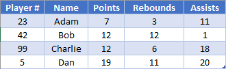
We want to find Bob’s Player #. Because the Player # is to the left of the name column, we can’t use a VLOOKUP.

Instead, we could do a basic MATCH request to calculate Bob’s row

=MATCH(H2, B2:B5, 0)

This will look for an exact match of the word “Bob”, and so our function would return the number 2, since “Bob” is in the 2^nd position.

Next we can use the INDEX Function to return the Player #, corresponding to a row. For now, let’s just manually enter “2” into the function:

=INDEX(A2:A5, 2)

Here, INDEX will reference A3, since that’s the 2^nd cell within the A2:A5 range and return the result of 42. For our overall goal, we can then combine these two into:

=INDEX(A2:A5, MATCH(H2, B2:B5, 0))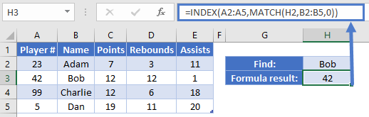

The benefit here is that we were able to return a result from a column to the left of where we were searching.

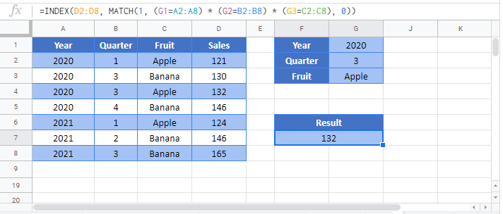
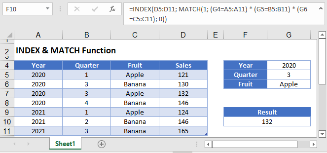
Two-dimension lookup

Let’s look at our table from before:

This time however, we want to fetch a specific statistic. We’ve called out that we want to search for Rebounds in cell H1. Rather than having to write several IF statements to determine which column to get the result from, you can use a MATCH function again. The INDEX function lets you specify the row value and the column value. We’re going to add another MATCH function here to determine which column we want. That will look like

=MATCH(H1, A1:E1, 0)

Our cell in H1 is a dropdown that let’s us choose what category we want to search for, and then our MATCH determines which column in the table that belongs to. Let’s plug this new bit into our previous formula. Note that we need to tweak the first argument to be two dimensions, as we no longer just want a result from column A.

=INDEX(A2:E5, MATCH(H2, B2:B5, 0), MATCH(H1, A1:E1, 0))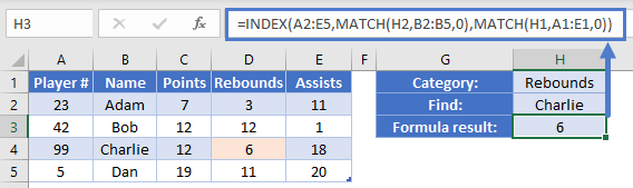

In our example, we want to find Rebounds for Charlie. Our formula is going to evaluate this like so:

=INDEX(A2:E5, MATCH("Charlie", B2:B5, 0), MATCH("Rebounds", A1:E1, 0))
=INDEX(A2:E5, 3, 4)
=D4
=6

We’ve now created a flexible setup that allows the user to fetch any value they want from our table without having to write multiple formulas or branching IF statements.

Multiple sections

It’s not often used, but INDEX has a fifth argument that can be given to determine which area within argument one to use. This means that we need a way to pass multiple areas into the first argument. You can do this by using an extra set of parentheses. This example will illustrate how you could fetch results from different tables on a worksheet using INDEX.

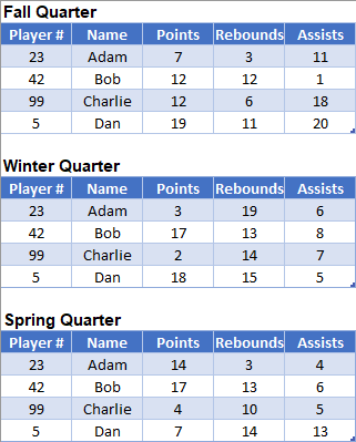
Here’s the layout we’ll be using. We’ve got statistics for three different quarters of play.

In cells H1:H3, we’ve created Data Validation drop down lists for our various choices. The dropdown for the Quarter is coming from J2:J4. We’ll use this for another MATCH statement, to determine which area to use. Our formula in H4 is going to look like this:

=INDEX((A3:E6, A10:E13, A17:E20), MATCH(H2, B3:B6, 0), MATCH(H1, A2:E2, 0), MATCH(H3, J2:J4, 0))

We’ve already discussed how the inner two MATCH functions work, so let’s focus on the first and last arguments:

=INDEX((A3:E6, A10:E13, A17:E20), …, MATCH(H3, J2:J4, 0))

We’ve given the INDEX function multiple arrays in the first argument by enclosing them all within parentheses. The other way you could do this is by using Formulas – Define Name. You could define a name called “MyTables” with a definition of:

='Multiple Sections'!$A$3:$E$6;'Multiple Sections'!$A$10:$E$13;'Multiple Sections'!$A$17:$E$20

This way, we are getting the follwing formula:

=INDEX(MyTable,MATCH(H2,Table1347[Name],0),MATCH(H1,Table1347[#Headers],0),MATCH(H3,J2:J4,0))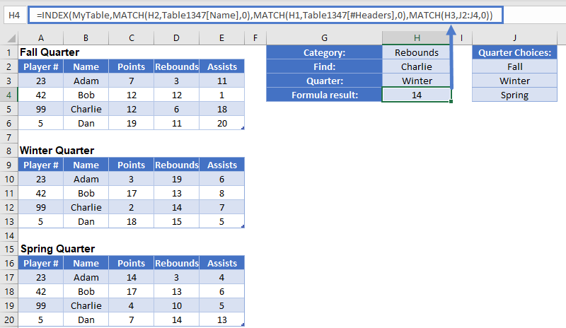

Let’s go back to the whole statement. Our various MATCH functions are going to tell the INDEX function exactly where to look. First, we’ll determine that “Charlie” is the 3^rd row. Next, we want “Rebounds”, which is the 4^th column. Finally, we’ve determined that we want the result from 2^nd table. The formula will evaluate through this like so:

=INDEX((A3:E6, A10:E13, A17:E20), MATCH(H2, B3:B6, 0), MATCH(H1, A2:E2, 0), MATCH(H3, J2:J4, 0))
=INDEX((A3:E6, A10:E13, A17:E20), 3, 4, 2)
=INDEX(A10:E13, 3, 4)
=D13
=14

As we mentioned at the beginning of this example, you’re limited to having the tables be on the same worksheet. If you can write out correct ways to tell your INDEX which row, column, and/or area you want to retrieve data from, INDEX will serve you very well.

Google Sheets –INDEX & MATCH

All of the above examples work exactly the same in Google Sheets as in Excel.