Non-Volatile Function Solutions in Excel
Written by
Reviewed by
Download the example workbook
Non-Volatile Solutions
We’ve discussed in other articles about how there are functions like OFFSET and INDIRECT which are volatile. If you start using many of these in a spreadsheet or have many cells dependent upon volatile function, you can cause your computer to spend a noticeable time doing recalculations every time you try to change a cell. Rather than becoming frustrated at how your computer isn’t fast enough, this article will explore alternative ways to solve the common situations people use OFFSET and INDIRECT.
Replacing OFFSET to create a dynamic list
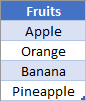
After learning about the OFFSET function, it’s a common misconception that it’s the only way to return a result with dynamic size using the last couple of arguments. Let’s look at a list in column A where our user might decide later to add additional items.
To make a dropdown in cell C2, you could define a Named Range with a volatile formula like
=OFFSET($A$2, 0, 0, COUNTA($A:$A)-1, 1)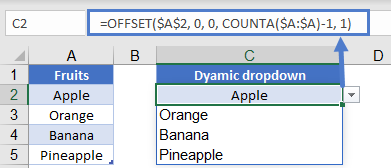
With the current setup, this would certainly return a reference to the range A2:A5. However, there’s another way using the non-volatile INDEX. To do this, think about we write a reference to the range going from A2 through A5. When you write “A2:A5”, don’t think of this as a single piece of data, but rather as a “StartingPoint” and “EndingPoint” separated by a colon (e.g., StartingPoint:EndingPoint). In a formula, both the StartingPoint and EndingPoint can be the results of other functions.
Here’s the formula we’ll use to create out dynamic range using the INDEX Function:
=$A$2:INDEX($A:$A, COUNTA($A:$A))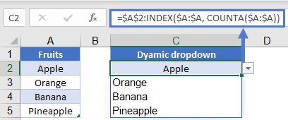
Note that we’ve stated that the StartingPoint for this range will always be A2. On the other side of the colon, we’re using INDEX to determine where the EndingPoint shall be. The COUNTA will determine that there are 5 cells with data in column A, and so our INDEX will create a reference to A5. The formula thus gets evaluated like so:
=$A$2:INDEX($A:$A, COUNTA($A:$A))
=$A$2:INDEX($A:$A, 5)
=$A$2:$A5
Using this technique, you can dynamically build a reference to any list, or even a two-dimensional table using the INDEX function. In a spreadsheet with an abundance of OFFSET functions, replacing the OFFSETs with INDEX will allow your computer to start running much faster.
Replacing INDIRECT for sheet names
The INDIRECT function often gets called when workbooks have been designed with data scattered across multiple worksheets. If you can’t get all the data onto a single sheet, but don’t want to use a volatile function, you might be able to use CHOOSE.
Consider the following layout, where we have Sales data across 3 different worksheets. On our Summary sheet, we’ve selected which quarter we’d like to view the data from.
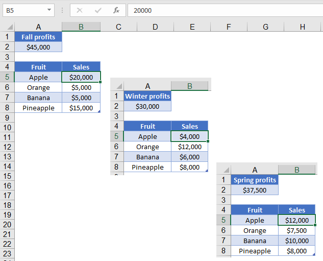
Our formula in B3 is:
=CHOOSE(MATCH(B2, D2:D4, 0), Fall!A2, Winter!A2, Spring!A2)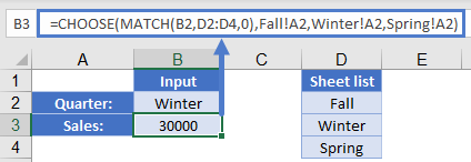
In this formula, the MATCH function is going to determine which area we want to return. This then tells the CHOOSE function which of the following ranges to return as the result.
You can also use the CHOOSE function to return a larger range. In this example, we’ve got a table of sales data on each of our three worksheets.
Rather than writing an INDIRECT function to build the sheet name, you can let CHOOSE determine which table to do the search on. In my example, I’ve already named the three tables tbFall, tbWinter, and tbSpring. The formula in B4 is:
=VLOOKUP(B3, CHOOSE(MATCH(B2, D2:D4, 0), tbFall, tbWinter, tbSpring), 2, 0)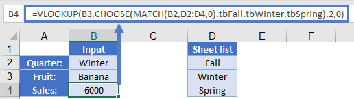
In this formula, the MATCH is going to determine that we want the 2nd item from our list. CHOOSE will then take that 2 and return the reference to tbWinter. Finally, our VLOOKUP will be able to complete the search in the given table, and it will find that the total sales for Banana in winter was $6000.
=VLOOKUP(B3, CHOOSE(MATCH(B2, D2:D4, 0), tbFall, tbWinter, tbSpring), 2, 0)
=VLOOKUP(B3, CHOOSE(2, tbFall, tbWinter, tbSpring), 2, 0)
=VLOOKUP(B3, tbWinter, 2, 0)
=6000
This technique is limited by the fact that you must fill out the CHOOSE function with all the areas you might want to fetch a value from, but it does give you the benefit of avoiding a volatile formula. Depending on how many calculations you need to complete, this ability could prove to be quite valuable.

