OFFSET Function Examples – Excel & Google Sheets
Written by
Reviewed by
Download the example workbook
This Tutorial demonstrates how to use the Excel OFFSET Function in Excel and Google Sheets to create a reference offset from an initial cell.
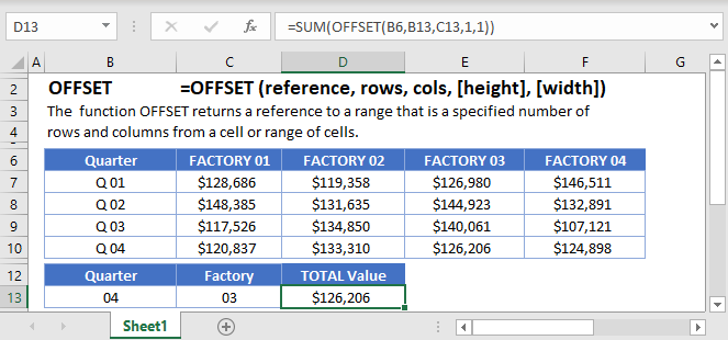
OFFSET Function Overview
The OFFSET Function Starts with a defined cell reference and returns a cell reference a specificed number of rows and columns offset from the original referece. References can be one cell or a range of cells. Offset also allows you to resize the reference a given number of rows/columns.
(Notice how the formula inputs appear)
IFERROR Function Syntax and Inputs:
=OFFSET(reference,rows,cols,height,width)reference – The initial cell reference from which you want to offset.
rows – The number of rows to offset.
cols – The number of columns to offset.
height – OPTIONAL: Adjust the number of rows in the reference.
width – OPTIONAL: Adjust the number of columns in the reference.
What is the OFFSET function?
The OFFSET function is one of the more powerful spreadsheet functions as it can be quite versatile in what it creates. It gives the user the ability to define a cell or range in a variety of position and sizes.
CAUTION: The OFFSET function is one of the volatile functions. Most of the time when you’re working in your spreadsheet, the computer will only recalculate a formula if the inputs have changed their values. A volatile function, however, recalculates every time you make a change to any cell. Caution should be used to ensure that you don’t cause a large recalculation time due to excessive use of volatile function or having many cells dependent upon the result of a volatile function.
Basic Row Examples
In every use of the OFFSET function, you need to give a starting point, or anchor. Let’s look at this table to help understand this:
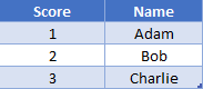
We’ll use “Bob” in cell B3 as our anchor point. If we wanted to grab the value just below (Charlie), we would say that we want to shift the row by 1. Our formula would look like
=OFFSET(B3, 1)If we wanted to shift up, that would be a negative shift. You can think of this as the row number is decreasing, so we need to subtract. Thus, to get the value above (Adam), we would write
=OFFSET(B2, -1)Basic Column Examples
Continuing the idea from previous example, we’ll add another column to our table.
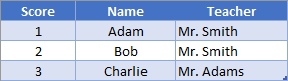
If we wanted to grab the teacher for Bob, we could use the formula
=OFFSET(B2, 0, 1)In this instance, we said that we want to offset zero rows (aka stay on same row) but we want to offset 1 column. For columns, a positive number means to offset to the right, and negative numbers mean to offset to the left.
OFFSET and MATCH
Suppose you had several columns of data, and you wanted to give the user the ability to choose which column to fetch results from. You could use the INDEX function, or you can use OFFSET. Since MATCH will return the relative position of a value, we’ll need to make sure the anchor point is to the left of our first possible value. Consider the following layout:
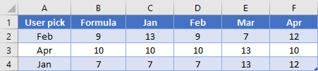
In B2, we’ll write this formula:
=OFFSET(B2, 0, MATCH(A2, $C$1:$F$1, 0))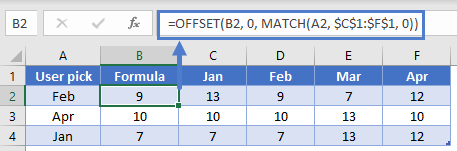
The MATCH is going to look “Feb” in the range C1:F1 and find it in the 2nd cell. The OFFSET will then shift 1 column to the right of B2 and grab the desired value of 9. Note that OFFSET has no problem using the same cell that contains the formula as the anchor point.
NOTE: This technique could be used as a replacement to VLOOKUP or HLOOKUP when you want to return a value from the left/above your lookup range. This is because OFFSET can do negative offsets.
OFFSET to get a range
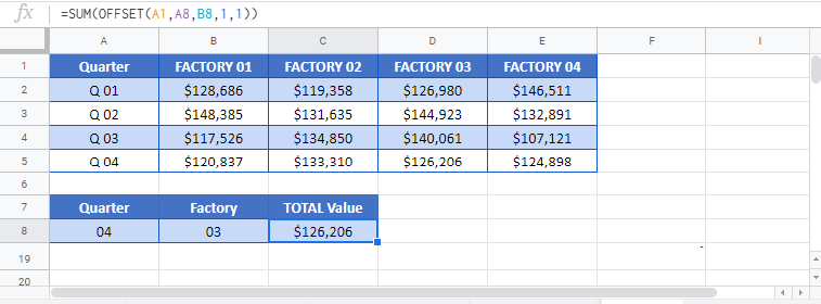
You can use the 4th and 5th arguments in the OFFSET function to return a range rather than just a single cell. Suppose you wanted to sum 3 columns in this table.
=AVERAGE(OFFSET(A1,MATCH(F2,A2:A5,0),1,1,3))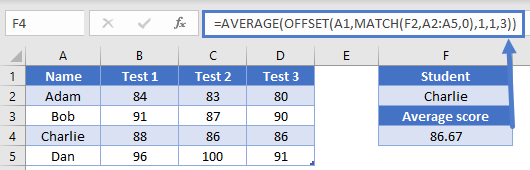
In F2, we’ve selected the name of a student that we want to fetch their average test scores for. To do this, we’ll use the formula
=AVERAGE(OFFSET(A1,MATCH(F2,A2:A5,0),1,1,3))The MATCH is going to search through column A for our name and return the relative position, which is 3 in our example. Let’s see how this will get evaluated. First, the OFFSET is going to go down 3 rows from A1, and 1 column to the right from A1. This places us in cell B3.
=AVERAGE(OFFSET(A1, 3, 1, 1, 3))Next, we’re going to resize the range. The new range will have B3 as top left cell. It will be 1 row high and 3 columns high, giving us the range B4:D4.
=AVERAGE(OFFSET(A1,3, 1, 1, 3))Note that while you can legitimately put negative values in the offset arguments, you can only use non-negative values in the sizing arguments.
At the end, our AVERAGE function sees:
=AVERAGE(B4:D4)Thus, we get our solution of 86.67
OFFSET with dynamic SUM
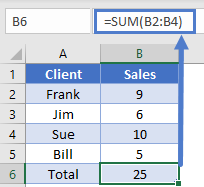
Because OFFSET is used to find a reference, rather than pointing to the cell directly, it’s most helpful when you are dealing with data that has rows added or deleted. Consider the following table with a Total at the bottom
=SUM(B2:B4)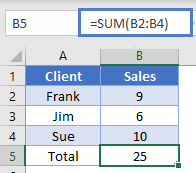
If we had used a basic SUM formula here of “=SUM(B2:B4)” and then inserted a new row to add a record for Bill, we would have the wrong answer
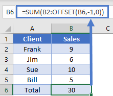
Instead, let’s think of how to solve this from the Total’s view point. We really want to grab everything from cell B2 to the cell just above our total. The way we can write this in a formula is to do a row offset of -1. Thus, we use this as the formula for our total in cell B5:
=SUM(B2:OFFSET(B5,-1,0))This formula does what we just described: start at B2 and go to 1 cell above our total cell. You can see how after adding Bill’s data, our total gets updated correctly.
OFFSET to get last N items
Let’s say that you are recording monthly sales but want to be able to look at the last 3 months. Rather than having to manually update your formulas to keep adjusting as new data is added, you can use the OFFSET function with COUNT.
We’ve already shown how you can use OFFSET to grab a range of cells. To determine how many cells we need to shift, we’ll use COUNT to find how many numbers are in column B. Let’s look at our sample table.
=SUM(OFFSET($B$1,COUNT(B:B)-$E$1+1,0,$E$1,1))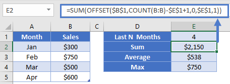
If we started at B1 and offset 4 rows (the count of numbers in column B), we’d end up at the bottom of our range, B5. However, since OFFSET can’t resize with a negative value, we need to do some adjustments so that we end up in B3. The general equation for this is going to be to do
COUNT(…) – N + 1We take the count of entire column, subtract however many we want to return (since we’ll resize to grab them), and then add 1 (since we’re essentially starting our offset at position zero).
Here you can see we’ve setup a range to get the Sum, Average, and Max of last N months. In E1, we’ve entered the value of 3. In E2, our formula is
=SUM(OFFSET($B$1,COUNT(B:B)-$E$1+1,0,$E$1,1))The highlighted section is our general equation that we just discussed. We don’t need to offset any columns. We’re then going to resize the range to be 3 cells tall (determined by the value in E1) and 1 column wide. Our SUM then takes this range and gives us the result of $1,850. We’ve also shown that you can calculate the average of max of this same range by simply switching the outer function from SUM to whatever the situation requires.
OFFSET dynamic validation lists
Using the technique shown in last example, we can also build Named Ranges that could be used in Data Validation or charts. This can be helpful when you want to setup a spreadsheet but are expecting our lists/data to change size. Let’s say that our store is starting to sell fruit, and we currently have 3 choices.
<Note – insert image>
<From Indika To Steve- Note from article – Note to Steve: Might need some gifs here, or snapshopts of cells w/ dropdown showing>
To make a Data Validation dropdown that we can use elsewhere, we’ll define the named range MyFruit as
=$A$2:OFFSET($A$1, COUNTA($A:$A)-1, 0)Instead of COUNT, we’re using COUNTA since we are dealing with text values. Because of this though, our COUNTA is going to be one higher since it’s going to count the header cell in A1 and give a value of 4. If we offset by 4 rows though, we’d end up in cell A5 which is blank. To adjust for this then, we subtract the 1.
Now that we’ve got our Named Range setup, we can setup some Data Validation in cell C4 by using a List type, with source:
=MyFruitNote that the dropdown only shows our three current items. If we then add more items to our list and go back to the dropdown, the list shows all the new items without us having to change any of the formulas.
Cautions with using OFFSET
As mentioned at the beginning of this article, OFFSET is a volatile function. You won’t notice this if you’re using it in just a few cells, but if you start having it involved in hundreds of calculations and you’ll quickly notice your computer spending a noticeable amount of time recalculating every time you make any changes.
Additionally, because OFFSET doesn’t’ directly name the cells it’s looking at, it is harder for other users to come by later and change your formulas if need be.
Instead, it would be advisable to use Tables (introduced in Office 2007) which allow structural references. These helped users be able to give a single reference that automatically adjusted in size as new data was added or deleted.
The other option to use instead of OFFSET is the powerful INDEX function. INDEX lets you build all the dynamic ranges we saw in this article without the issue of being a volatile function.
Additional Notes
Use the OFFSET Function to return a cell value (or a range of cells) by offsetting a given number of rows and columns from a starting reference. When looking only for a single cell, OFFSET formulas achieve the same purpose as the INDEX Formulas, using a slightly different technique. The real power of the OFFSET Function lies in its ability to select a range of cells to be used in another formula.
When using the OFFSET Function, you define an initial starting cell or range of cells. Then you indicate the number of rows and columns to offset from that initial cell. You can also resize the range; add or subtract rows or columns.
Return to the List of all Functions in Excel
OFFSET in Google Sheets
The OFFSET Function works exactly the same in Google Sheets as in Excel: