Search by Keywords – Excel & Google Sheets

This tutorial will demonstrate how to search by keywords in Excel and Google Sheets.

Search by Keywords

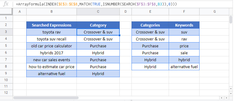
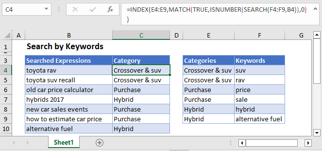
To categorize text cells based on the keywords they contain, you can use the SEARCH, ISNUMBER, MATCH, and INDEX Functions combined.

=INDEX(E3:E8,MATCH(TRUE,ISNUMBER(SEARCH(F3:F8,B3)),0))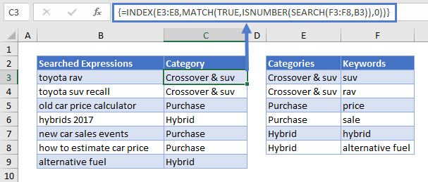

Note: This is an array formula. When using Excel 2019 and earlier, you must enter the array formula by pressing CTRL + SHIFT + ENTER (instead of ENTER), telling Excel that the formula in an array formula. You’ll know it’s an array formula by the curly brackets that appear around the formula (see top image). In later versions of Excel and Excel 365, you can simply press ENTER instead.

Let’s see how this formula works.

SEARCH Function

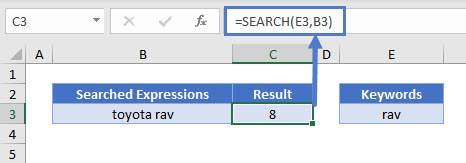
Typically, the  SEARCH Function looks for a string of text inside a cell value, returning the position where the text is found.

 

However, if you use an array formula, and enter an array of values to search for, the SEARCH Function will return an array of matches.

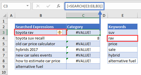
As shown above, For cell B3 (“toyota rav”), it will return an array like this:

{#VALUE, 8, #VALUE, #VALUE, #VALUE, #VALUE}

meaning that it found only one of the keywords (“rav”) in the string, at position 8.

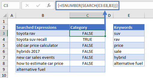
ISNUMBER Function

The ISNUMBER Function translates the array given by the SEARCH Function to TRUE and FALSE values.

 

MATCH Function

With the MATCH Function, we find the position of the TRUE value in our ISNUMBER array from above.

=MATCH(TRUE,ISNUMBER(SEARCH(F3:F8,B3)),0)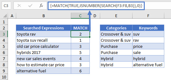

For “toyota rav,” the TRUE is the second value in the array.

INDEX Function

Finally, we use the result of the MATCH Function to determine which Category row we need with the INDEX Function.

=INDEX(F3:F8,C3)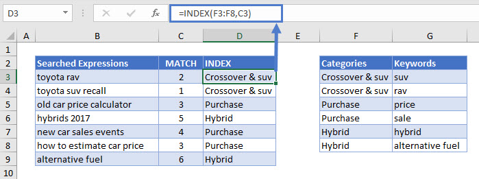

The second row of the Categories list is “Crossover & suv,” so that’s the matching Category for “toyota rav.”

Replacing “C3” with the MATCH expression brings us back to our original formula:

=INDEX(E3:E8,MATCH(TRUE,ISNUMBER(SEARCH(F3:F8,B3)),0))

 

Reminder: This is an array formula. When using Excel 2019 and earlier, you must enter the array formula by pressing CTRL + SHIFT + ENTER (instead of ENTER), telling Excel that the formula in an array formula. You’ll know it’s an array formula by the curly brackets that appear around the formula (see top image). In later versions of Excel and Excel 365, you can simply press ENTER instead.

Search by Keywords in Google Sheets

These formulas work exactly the same in Google Sheets as in Excel.