Sum If Not Blank – Excel & Google Sheets
Written by
Reviewed by
Download the example workbook
This tutorial will demonstrate how to use the SUMIFS Function to sum data related to non-blank or non-empty cells in Excel and Google Sheets.
Sum if Not Blank
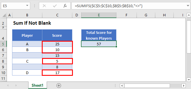
First, we will demonstrate how to sum data relating to non-blank cells.
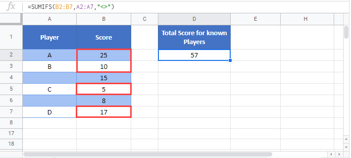
We can use the SUMIFS Function to sum all Scores for Players with non-blank names using criteria (“<>”).
=SUMIFS(C3:C8,B3:B8,"<>")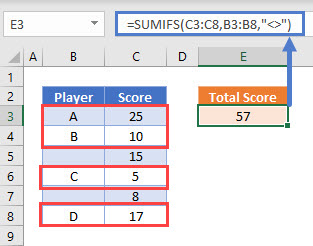
Treating Spaces as Blank Cells – With Helper Column
You need to be careful when interacting with blank cells in Excel. Cells can appear blank to you, but Excel won’t treat them as blank. This can occur if the cell contains spaces, line-breaks, or other invisible characters. This is a common problem when importing data into Excel from other sources.
If we need to treat any cells that only contain spaces the same way as if they were blank, then the formula in the previous example will not work. Notice how the SUMIFS Formula does not consider cell B9 below (” “) to be blank:
=SUMIFS(D3:D9,B3:B9,"<>")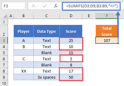
To treat a cell containing only spaces as if it were a blank cell, we can add a helper column using the LEN and TRIM Functions..
The TRIM Function removes the extra spaces from the cell.
The LEN Function counts the number of remaining characters. If the count is 0, then the “trimmed” cell is blank.
=LEN(TRIM(B3))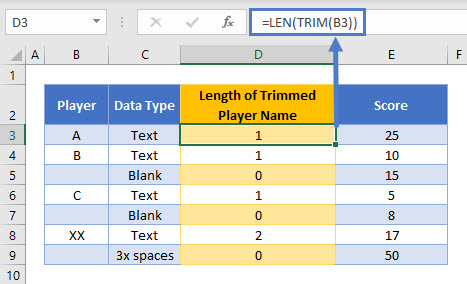
Now use the SUMIFS Function to sum if count > 0.
=SUMIFS(E3:E9,D3:D9,">0")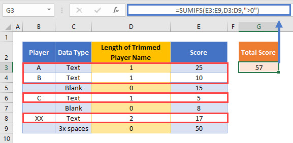
The helper column is easy to create and easy to read, but you might wish to have a single formula to accomplish the task. This is covered in the next section.
Treating Spaces as Blank Cells – Without Helper Column
To accomplish all this with a single formula, we can use the SUMPRODUCT Function in combination with the LEN and TRIM Functions.
=SUMPRODUCT(--(LEN(TRIM(B3:B9))>0),D3:D9)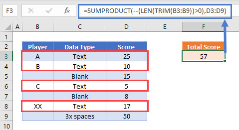
Let’s walk through the formula.
First, the SUMPRODUCT Function reads the cell values:
=SUMPRODUCT(--(LEN(TRIM({"A"; "B"; ""; "C"; ""; "XX"; " "}))>0),{25; 10; 15; 5; 8; 17; 50})Then, the TRIM Function removes leading and trailing spaces from Player names:
=SUMPRODUCT(--(LEN({"A"; "B"; ""; "C"; ""; "XX"; ""})>0),{25; 10; 15; 5; 8; 17; 50})The LEN Function calculates the lengths of the trimmed Player names:
=SUMPRODUCT(--({1; 1; 0; 1; 0; 2; 0}>0),{25; 10; 15; 5; 8; 17; 50})With the logical test (>0), any trimmed Player names with more than 0 characters are changed to TRUE:
=SUMPRODUCT(--({TRUE; TRUE ; FALSE; TRUE; FALSE; TRUE; FALSE}),{25; 10; 15; 5; 8; 17; 50})Next the double dashes (–) convert the TRUE and FALSE values into 1s and 0s:
=SUMPRODUCT({1; 1; 0; 1; 0; 1; 0},{25; 10; 15; 5; 8; 17; 50})The SUMPRODUCT Function then multiplies each pair of entries in the arrays to produce an array of Scores only for Player names that are not blank or not made only from spaces:
=SUMPRODUCT({25; 10; 0; 5; 0; 17; 0})Finally, the numbers in the array are summed together
=57More details about using Boolean statements and the “–” command in a SUMPRODUCT Function can be found here
Sum if Not Blank in Google Sheets
These formulas work exactly the same in Google Sheets as in Excel.