Two Dimensional VLOOKUP
Written by
Reviewed by
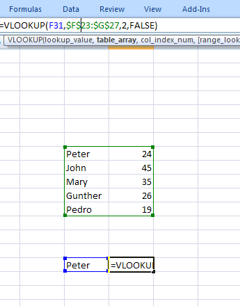
The VLOOKUP and HLOOKUP functions are well known for looking up data in one dimension:
And then:
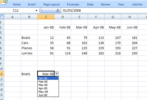
However what happens if we have a TWO dimensional array
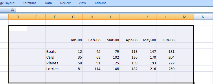
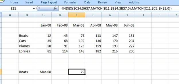
And we want to find the value for Boats in Mar-08. So we could add two drop downs to specify the mode of transport and the month that we need:
Excel provides a function called INDEX that allows us to return values from a 2d array:
INDEX(Array_Range, Row Number, Col Number)
Where
• Array_Range is the range in Excel of the two dimensional array – in this case $B$4:$H$7
• Row Number is the position in the list where we find the text “Boat” – in this case is 1
• Col Number is the position in the list where we find the month “Mar-08”
Of course the only thing left to do is to determine the Row and Column Number. This is done by using the MATCH function – which returns the position of a string within a range of values:
MATCH(“String”, Range,0) – will return the position of “String” in the array “Range” and the 0 states that we want an exact match. So we are looking for the position of Boats in the range {Boats, Cars, Planes , Lorries} – which is 1. This will give the row number:
MATCH(B11,$B$4:$B$7,0)
And similarly for the column number
MATCH(C11,$C$2:$H2,0)
And then we combine all these into one function:
=INDEX($C$4:$H$7,MATCH(B11,$B$4:$B$7,0),MATCH(C11,$C2:$H$2,0))
To give the value of 79 for boats in March 2008: