Using Dynamic Ranges – Year to Date Values

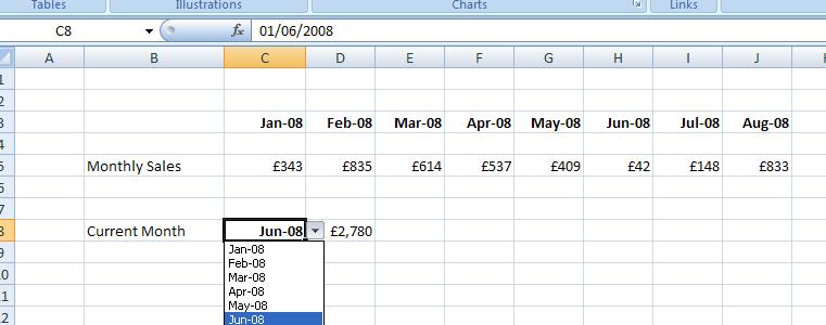
Imagine that we have some Sales Figures for a company:

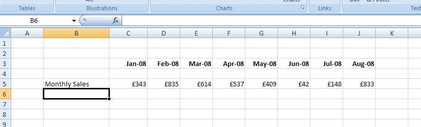
And that we wish to find the Total figures for the year to date. We can add a drop down like so:

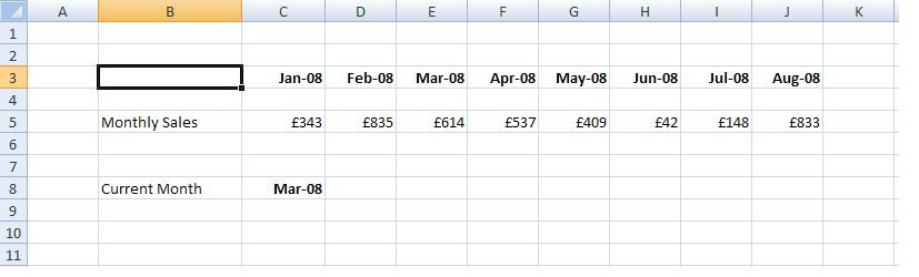
So that we can specify the current month. Hence we now want to work out the year to date for March. The simplest format would be to have a formulae that extended across the range:

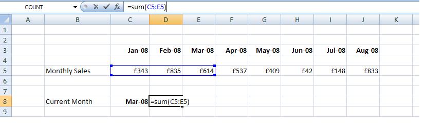
And then we would just change the formulae every month.

However Excel permits another approach. We could set up a dynamic range whose size varied on the month that we are in. As we change the month in the drop down then the size of the range changes.
So for the month of March the range is 3 columns long, and for the month of June it would be 6 months along.

The size of the range is governed by the month. One way of formulating this is to use the Month function:

=Month(c8)

Where c8 is the cell address of our drop down. However the method that is preferred is to use the MATCH function to determine the position of the current months in all the months in our report:

MATCH(c8,$c$3:$j$3,0)

Where:
• c8 is the cell address of the current month
• C3:J3 is the address of all our months
• 0 is to ensure an exact match

Now we can specify the size of our dynamic range by the OFFSET function which has 5 arguments:
=OFFSET(reference, rows, cols, height, width)

Where:
• Reference is the top left hand corner of our dynamic range – cell C5 – the first cell that we want to sum
• Rows – the number of rows down from our base cell – this is 0
• Cols – the number of cols across from our base call – this is 0
• The width of our dynamic range – which is 3 in this case. However as we wish the range to vary by month we will put our MATCH formulae here
• This is the height of our dynamic range which is 1

So our OFFSET formulae is:
= OFFSET(c5,0,0,MATCH(c8,$c$3:$j$3,0),1)

Finally we need to tell Excel to SUM this to give the complete formulae as:
= SUM(OFFSET(c5,0,0,MATCH(c8,$c$3:$j$3,0),1))

We have:

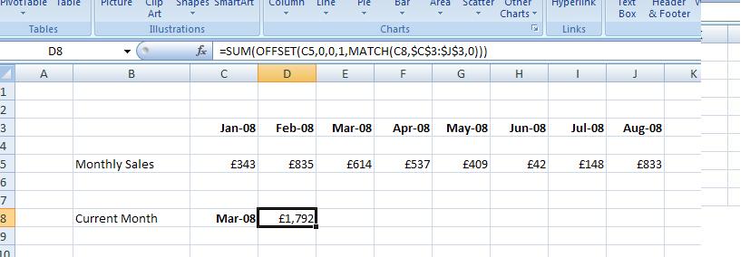
Now if we change the month in the dropdown, the correct year to date figure flows through:

As this is an automatic update this approach has the following advantages:
• There is no need to change the formulae each month
• As there are less formulae changes, less scope for error
• The spreadsheet can be used by somebody who has limited Excel knowledge – they can just change the dropdown and not be bothered by formulae