VLOOKUP Return Multiple Columns

This tutorial will demonstrate how to return multiple columns using VLOOKUP in Excel and Google Sheets. If your version of Excel supports XLOOKUP, we recommend using XLOOKUP instead.

 

VLOOKUP Array Formula

To VLOOKUP Multiple columns at once, you can create a single array formula (this section) or use helper columns (next section) if you don’t want to use an array formula.

 

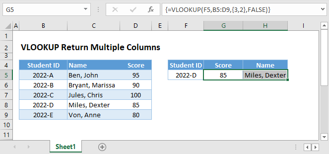
To VLOOKUP multiple columns at once with a single array formula, populate col_index_num with an array and convert the VLOOKUP Function to an array formula.

{=VLOOKUP(F3,B3:D7,{3,2},FALSE)}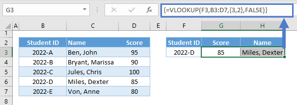

 

Let’s walk through the steps in creating the formula:

1. First, select the output range where the resulting array will be returned.

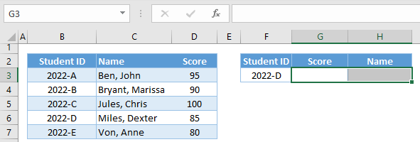
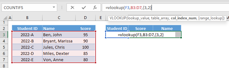
2. While the range is selected, we go to the formula bar and type our VLOOKUP Formula.

 

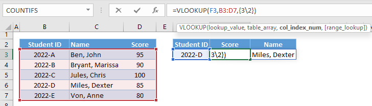
3. Next, we create our array input for col_index_num by enclosing the list of values with curly brackets ({}).

 

Note: To create a 1D Horizontal Array, we separate the values with a comma (,). For 1D Vertical Array, we use a semi-colon (;) as a separator. For 2D, we use a comma and semi-colon to imply a column and row, respectively.

For non-US Regional Settings, commas in formulas are replaced with semi-colons, and for arrays, we use the backslash (\) for columns and semi-colon (;) for rows:

4. Complete the formula and press Ctrl+Shift+Enter for Windows (Command+Return for Mac), and the curly brackets will automatically enclose the whole formula:

 

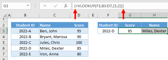
Note: These curly brackets signify an array formula, and unlike the curly brackets for the array of values, these curly brackets cannot be typed and can only be entered using the above method.

 

Instead of creating an array manually, we can reference the col_index_nums from a range. This makes it more dynamic compared to the previous method. We can do this with a single array formula:

{=VLOOKUP(F4,B3:D7,G2:H2,FALSE)}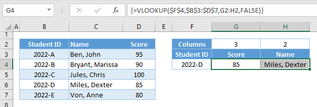

 

VLOOKUP non-Array Formula

If you don’t want to use an Array formula, you can set up “helper cells” for the column references and Copy and Paste the formula across multiple columns:

=VLOOKUP($F$4,$B$3:$D$7,G2,FALSE)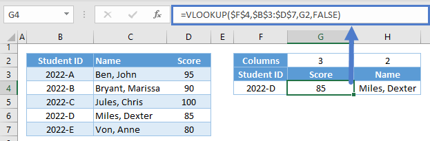

Note: Make sure to lock the cell references of lookup_value and table_array.

 

VLOOKUP-MATCH Dynamic Multiple Columns

By using VLOOKUP and MATCH together, you can dynamically lookup the column headers for the col_index_num:

=VLOOKUP($F$3,$B$3:$D$7,MATCH(G2,$B$2:$D$2,0),FALSE)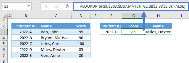

 

Google Sheets: VLOOKUP Return Multiple Columns

All formulas that were mentioned work the same way in Google Sheets, but for converting formulas to array formulas, Google Sheets has a function that is dedicated to doing this – the ARRAYFORMULA Function.

We can type ARRAYFORMULA or press Ctrl+Shift+Enter to automatically enclose our formula with the ARRAYFORMULA Function:

=ArrayFormula(VLOOKUP($F$3,$B$3:$D$7,MATCH(G2:H2,$B$2:$D$2,0),FALSE))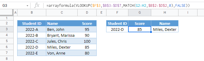

Note: No need to highlight the output range before entering the formula. The array formulas in Google Sheets are dynamic.