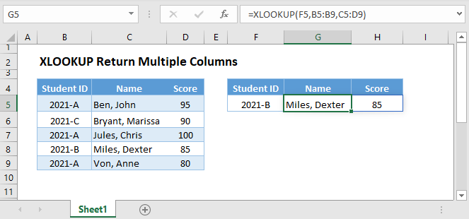
XLOOKUP Return Multiple Columns
Download the example workbook
This tutorial will demonstrate how to return multiple columns using XLOOKUP in Excel. If your version of Excel does not support XLOOKUP, read how to return multiple columns using VLOOKUP instead.
XLOOKUP Return Consecutive Columns
One advantage of the XLOOKUP Function is that it can return multiple consecutive columns at once. To do this, input the range of consecutive columns in the return array, and it will return all the columns.
=XLOOKUP(F3,B3:B7,C3:D7)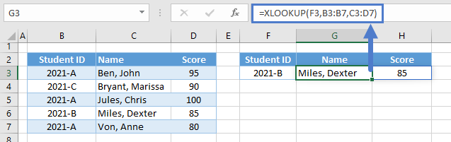
Notice here our return array is two columns (C and D), and thus 2 columns are returned.
XLOOKUP-FILTER Return Non-Adjacent Columns
Although the XLOOKUP Function can return multiple consecutive columns, it can’t return non-adjacent columns. To return non-adjacent columns, we can use the FILTER Function.
=XLOOKUP(F3,C3:C7,FILTER(B3:D7,{1,0,1}))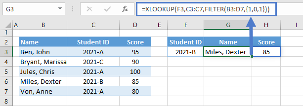
Let’s walk through the formula:
FILTER Function
The FILTER Function is commonly used for filtering rows, but it can also be used for filtering columns. To do this, we input a horizontal array of 1s (TRUE) and 0s (FALSE) with the same no. of columns from the array input (1st argument). Columns that match with 0s are filtered out while columns that match with 1s are returned.
=FILTER(B3:D7,{1,0,1})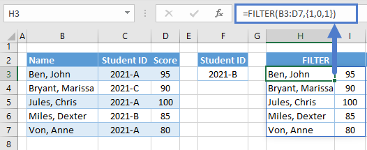
XLOOKUP Function
The output of the FILTER Function is then used as the return array of our XLOOKUP.
=XLOOKUP(F3,C3:C7,H3:I7)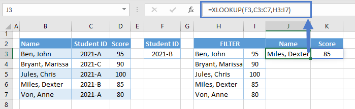
Combining all functions together yields our original formula:
=XLOOKUP(F3,C3:C7,FILTER(B3:D7,{1,0,1}))
XLOOKUP-FILTER-COUNTIF Return Non-Adjacent Columns
Instead of manually selecting the columns to be filtered out, we can use the COUNTIF Function to automatically determine the columns that will be returned and filtered out.
=XLOOKUP(F3,C3:C7,FILTER(B3:D7,COUNTIF(G2:H2,B2:D2)))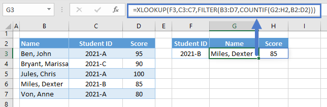
Let’s walk through the formula:
COUNTIF Function
First, let’s use the COUNTIF Function to count the instance of each source header (e.g., B2:D2) from the output headers (e.g., M2:N2).
=COUNTIF(M2:N2,B2:D2)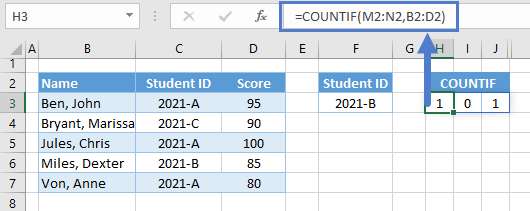
FILTER Function
The array result of the COUNTIF Function is then used as the filter condition to filter the columns.
=FILTER(B3:D7,H3:J3)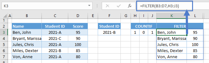
XLOOKUP Function
Finally, we can use the result of the FILTER Function in the XLOOKUP Function to return the columns that we want.
=XLOOKUP(F3,C3:C7,K3:L7)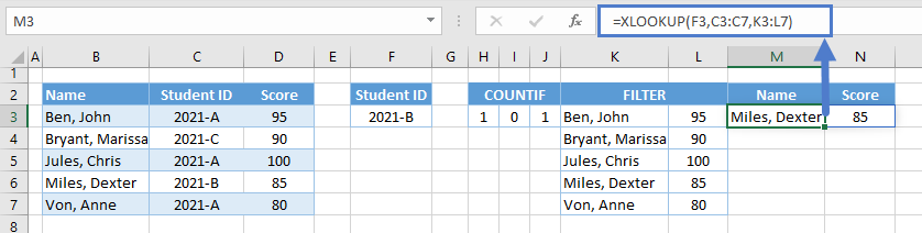
Combining all functions together yields our original formula:
=XLOOKUP(F3,C3:C7,FILTER(B3:D7,COUNTIF(G2:H2,B2:D2)))
XLOOKUP-CHOOSE Return Columns in Different Order
The XLOOKUP-FILTER-COUNTIF Formula can return non-adjacent columns, but what if we want to return any column in a different order? To solve this, let’s use the CHOOSE Function.
=XLOOKUP(F3,B3:B7,CHOOSE({2,1},C3:C7,D3:D7))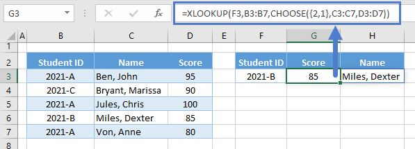
Let’s walk through the formula:
CHOOSE Function
First, we use the CHOOSE Function to join columns in a specified order into one array.
=CHOOSE({2,1},C3:C7,D3:D7)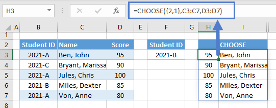
Note: We input the columns that we want separately in the CHOOSE Function (e.g., C3:C7, D3:D7), and we order them using the index_num (1st argument).
XLOOKUP Function
The resulting array from the CHOOSE Function is then used as the return array.
=XLOOKUP(F3,B3:B7,H3:I7)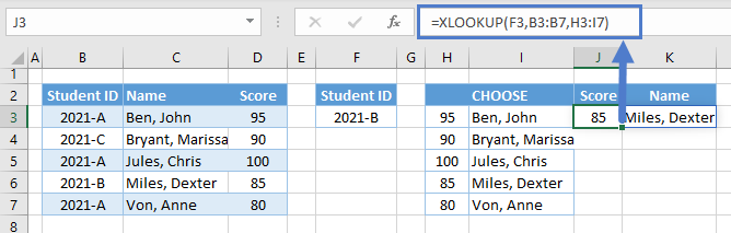
Combining all functions together yields our original formula:
=XLOOKUP(F3,B3:B7,CHOOSE({2,1},C3:C7,D3:D7))
XLOOKUP-CHOOSECOLS Return Columns in Different Order
The XLOOKUP-CHOOSE Formula becomes long and tedious if we have a lot of columns to return. Luckily, there’s a new array function (currently in the BETA Version of Excel 365) that is more convenient than CHOOSE Function – CHOOSECOLS Function.
=XLOOKUP(F3,B3:B7,CHOOSECOLS(B3:D7,3,2))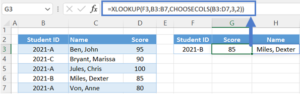
Let’s walk through the formula:
CHOOSECOLS Function
Unlike the CHOOSE Function where we join the columns in a specified order, the CHOOSECOLS Function returns the columns that we selected in the order that we specified.
=CHOOSECOLS(B3:D7,3,2)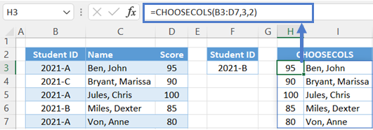
Note: The numbers that we specify in the col_num arguments (starting from the 2nd argument) are the relative column numbers of the columns from the given array (e.g., B3:D7).
XLOOKUP Function
Finally, we can use the XLOOKUP Function with the result of the CHOOSECOLS Function.
=XLOOKUP(F3,B3:B7,H3:I7)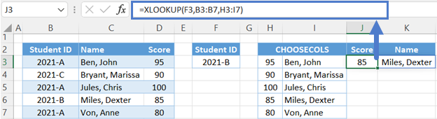
Combining all functions together yields our original formula:
=XLOOKUP(F3,B3:B7,CHOOSECOLS(B3:D7,3,2))
XLOOKUP-CHOOSECOLS-MATCH Return Columns in Different Order
Instead of manually selecting the columns and their order, we can use the MATCH Function to automatically determine the columns and their order that are required by the task.
=XLOOKUP(F3,B3:B7,CHOOSECOLS(B3:D7,MATCH(G2:H2,B2:D2,0)))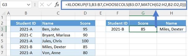
Let’s walk through the formula:
MATCH Function
First, we use the MATCH Function to determine the relative column positions of each output header from the source headers.
=MATCH(L2:M2,B2:D2,0)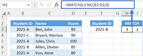
CHOOSECOLS Function
Now that we have the positions of the selected columns, we can use the CHOOSECOLS Function to return the selected columns in one array.
=CHOOSECOLS(B3:D7,H3:I3)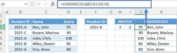
XLOOKUP Function
The last step is feeding the result of the CHOOSECOLS Function to the return array of the XLOOKUP Function.
=XLOOKUP(F3,B3:B7,J3:K7)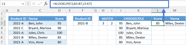
Combining all functions together yields our original formula:
=XLOOKUP(F3,B3:B7,CHOOSECOLS(B3:D7,MATCH(G2:H2,B2:D2,0)))
