XLOOKUP Multiple Criteria

This tutorial will demonstrate how to perform an XLOOKUP with multiple criteria in Excel. If your version of Excel does not support XLOOKUP, read how to use the VLOOKUP instead.

 

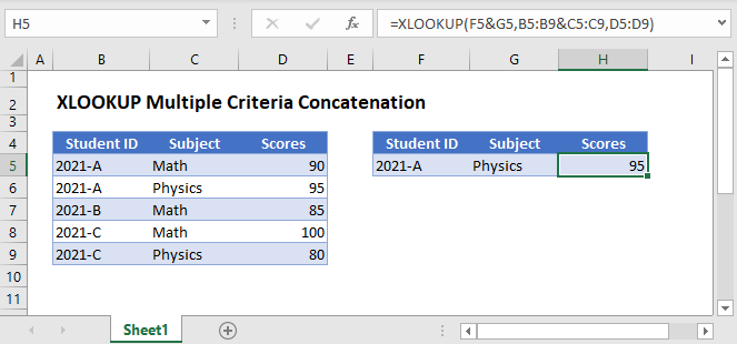
XLOOKUP Multiple Criteria Concatenation

One common way of performing a multiple criteria XLOOKUP is by concatenating all the criteria into one lookup value and their corresponding lookup columns into one lookup array.

=XLOOKUP(F3&G3,B3:B7&C3:C7,D3:D7)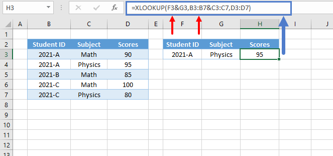

Let’s walk through the formula:

Concatenate the Lookup Columns

First, we concatenate the lookup columns to create an array of unique IDs, which enables us to look up all the criteria simultaneously.

=B3&C3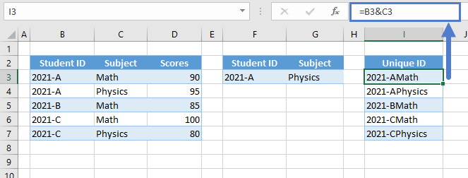

Concatenate the Criteria

Next, we also do the same for the criteria to create a new lookup value.

=F3&G3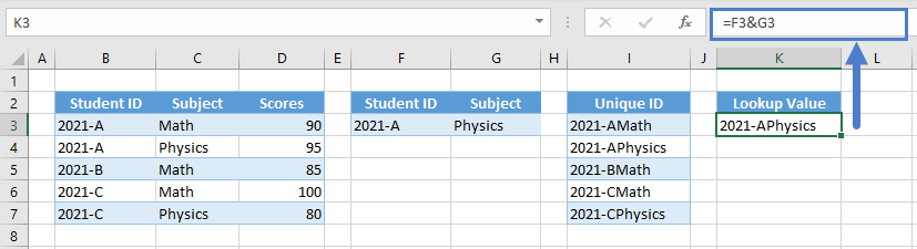

XLOOKUP Function

Finally, we supply the new lookup value and lookup array to the XLOOKUP Function.

=XLOOKUP(K3,I3:I7,D3:D7)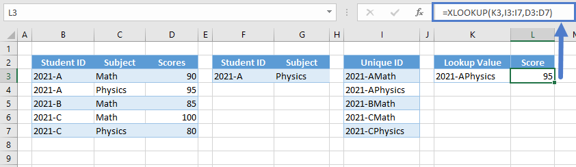

Putting it all together yields the original formula:

=XLOOKUP(F3&G3,B3:B7&C3:C7,D3:D7)

 

XLOOKUP Multiple Criteria Boolean Expressions

Another option is creating Boolean expressions where the criteria are checked against their corresponding lookup columns.

=XLOOKUP(1,(B3:B7=F3)*(C3:C7=G3),D3:D7)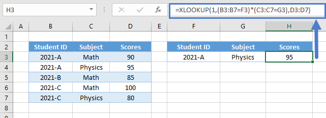

Let’s walk through this formula:

Boolean Expressions

First, let’s apply the appropriate criteria to their corresponding columns by using the logical operators (e.g., =,<,>).

Let’s start with the first criterion (e.g., Student ID).

=B3=$F$3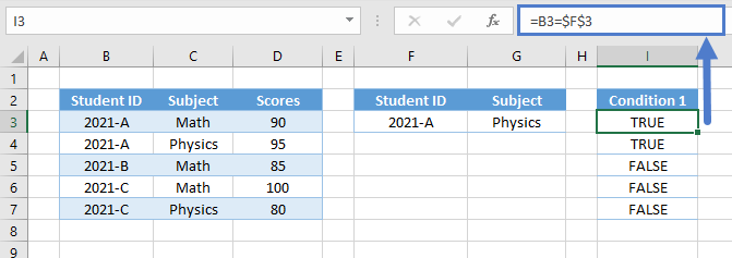

Repeat the step for the other criteria (e.g., Subject).

=C3=$G$3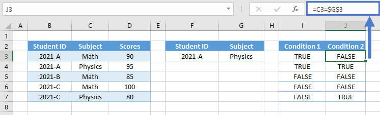

Array AND

Next, we perform the array equivalent of the AND Function by multiplying the Boolean arrays where TRUE is 1 and FALSE is 0.

=I3*J3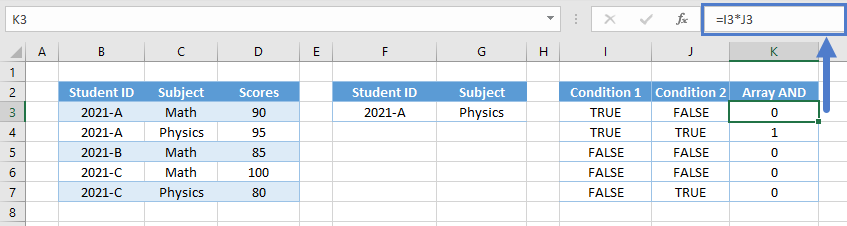

Note: The AND Function is an aggregate function (many inputs to one output). Therefore, we can’t use it in array calculations.

 

XLOOKUP Function

Next, we look up 1 from the result of the Array AND.

=XLOOKUP(1,K3:K7,D3:D7)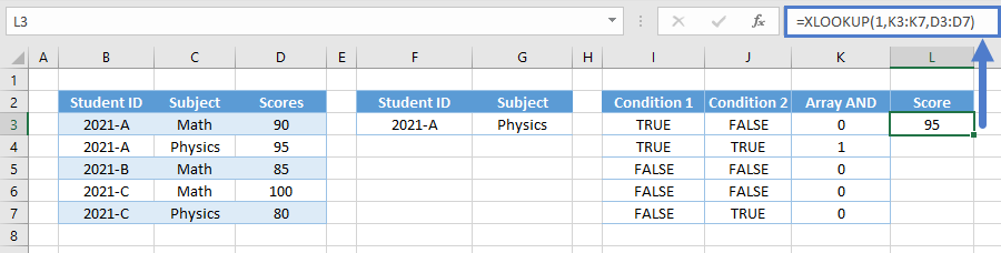

Combining all formulas yields our original formula:

=XLOOKUP(1,(B3:B7=F3)*(C3:C7=G3),D3:D7)