Top 11 Alternatives to VLOOKUP (Updated 2022!) – Excel & Google Sheets

This tutorial demonstrates the best VLOOKUP alternatives in Excel and Google Sheets.

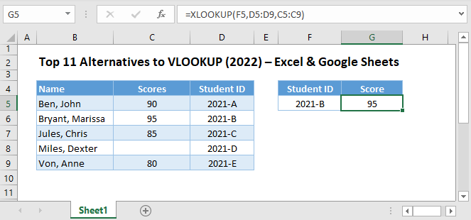
1. The XLOOKUP Function

If you have a new version of Excel, then the XLOOKUP Function is the best alternative to the VLOOKUP Function.

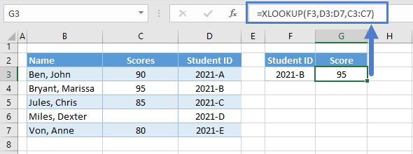
XLOOKUP: Left-Lookup

The lookup array and return array for the XLOOKUP Function are separate arguments. This leads to the following advantages:

1. No need to adjust the formula when columns are inserted or deleted.
2. No need to enter multiple column ranges/arrays when the lookup and return columns are not adjacent. This reduces the amount of data to be processed.
3. Being able to perform left-lookups (see example):

=XLOOKUP(F3,D3:D7,C3:C7)

XLOOKUP: Return more Columns

One feature of the XLOOKUP Function is being able to return more than one column.

=XLOOKUP(F3,B3:B7,C3:D7)

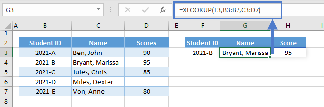
Note: The return array (columns) must be contiguous.

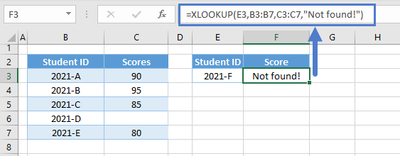
XLOOKUP: #N/A Error – Handling

Unlike the VLOOKUP Function where we need to use IFERROR or IFNA functions to handle the #N/A Error, the XLOOKUP Function has a built-in #N/A Error handler, which is the fourth argument (if_not_found).

=XLOOKUP(E3,B3:B7,C3:C7,"Not found!")

XLOOKUP: Match Mode Options

Another great feature of the XLOOKUP Function is being able to select match_mode (fifth argument): 0 – Exact Match, -1 – Exact Match or Next Smaller Item, 1 – Exact Match or Next Larger Item and 2 – Wildcard Character Match.

=XLOOKUP(E3,B3:B7,C3:C7,"No discount!",-1)

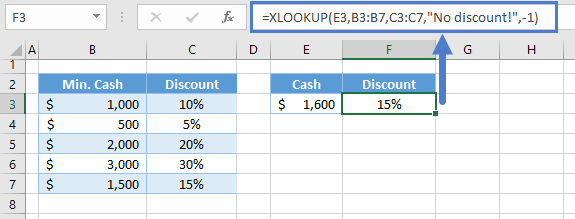
Note: Unlike the approximate matches from the VLOOKUP, LOOKUP, and MATCH Functions, where we need to sort the data, the XLOOKUP Function’s match_mode, by default, doesn’t require sorting of data (see example).

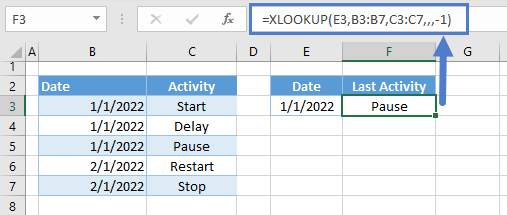
XLOOKUP: Last Lookup

The match_mode example from the previous section doesn’t require a sorted dataset because the default value of the search_mode (sixth argument) is a linear search (from first to last). Now, we can select the search process of our lookup (i.e., linear search and binary search), and one of these is the Search last-to-first option (i.e., -1), which enables us to easily return the last match.

=XLOOKUP(E3,B3:B7,C3:C7,,,-1)

XLOOKUP: Binary-Exact Match and Dynamic Arrays

The most important upgrade from the VLOOKUP Function or even the INDEX-MATCH Formula is being able to perform an exact match with a binary search process. We can now utilize the speed of the binary search without sacrificing exact matching by just setting the last argument, search_mode, to either 2 (Ascending Order) or -2 (Descending Order).

Let’s look at a one million lookup scenario:

=XLOOKUP(C3:C1000002,B3:B1000002,B3:B1000002,,,2)

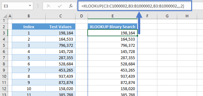
Note: By default, the match_mode is 0, which is Exact Match.

With the binary search, we can perform such lookup in less than 5 seconds. Another thing is that we can convert the XLOOKUP Function into a dynamic array formula. One way is to enter an array input in the lookup value (e.g., C3:C1000002).

2. INDEX-MATCH Formulas

The INDEX-MATCH Formula is the best-known alternative to the VLOOKUP Function in previous versions of Excel.

INDEX-MATCH: Left-Lookup

Just like with the XLOOKUP Function, the lookup column and return column are separated in INDEX-MATCH Formula. The lookup column is entered in the MATCH Function, which also performs the search process, while the return column is entered in the INDEX Function, which returns the value that corresponds to the result of the MATCH Function. This arrangement provides the same benefits mentioned in the XLOOKUP Function: automatic adjustment to column insertions and deletions, faster and efficient formula due to lesser column-array inputs and being able to perform left-lookups (see example below).

=INDEX(C3:C7,MATCH(F3,D3:D7,0))

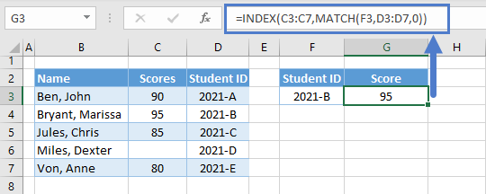
Let’s walk through the formula:

MATCH Function

Let’s start by finding the relative row coordinate of the lookup value (e.g., Student ID) from the lookup array (e.g., D3:D7) using the MATCH Function.

=MATCH(F3,D3:D7,0)

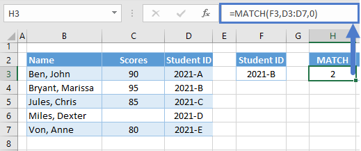
Note: The match_type (third argument) of the MATCH Function defines the match mode. Zero means exact match while 1 and -1 are both approximate matches.

INDEX Function

Once we have the row coordinate, we can now use this to return a value from the corresponding return array (e.g., C3:C7) using the INDEX Function.

=INDEX(C3:C7,H3)

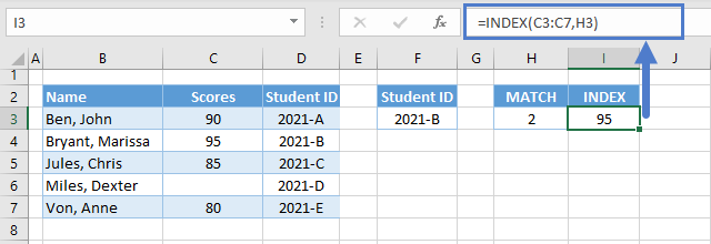
Note: The INDEX Function returns a value from an array given the relative row and column (for 2D array) coordinates.

Combining the two formulas yields our original formula:

=INDEX(C3:C7,MATCH(F3,D3:D7,0))

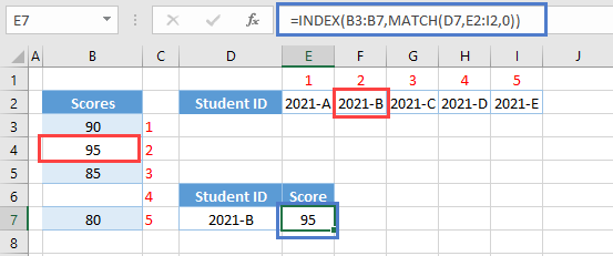
INDEX-MATCH: Horizontal Lookup Array

Another example that showcases the flexibility of the INDEX-MATCH Formula is when the lookup array and return array are in opposite orientations:

=INDEX(B3:B7,MATCH(D7,E2:I2,0))

3. The HLOOKUP Function

Now that we’re talking about horizontal orientations, there’s also a lookup function that is built for horizontal lookups – the HLOOKUP Function.

=HLOOKUP(I3,C2:G3,2,FALSE)

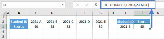
Note: The HLOOKUP Function works the same way as the VLOOKUP Function but in the opposite orientation. It searches the exact match in the first row and returns the corresponding value from a given row_index_num.

4. OFFSET-MATCH Formulas: Dynamic Column Reference

Another alternative to VLOOKUP is the OFFSET-MATCH Formula, which works similarly to the INDEX-MATCH Formula.

Let’s look at a lookup with dynamic column reference scenario and see how the OFFSET slightly differs from the INDEX-MATCH.

=OFFSET(B2,MATCH(F3,B3:B7,0),MATCH(G3,C2:D2,0))

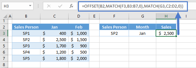
Let’s walk through the formula:

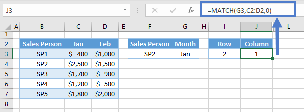
Row and Column Coordinates

First, we need to determine the relative row and column coordinates using the MATCH Function.

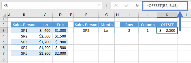
OFFSET Function

Instead of using the INDEX Function to return a value, we’ll replace it with the OFFSET Function. By default, the OFFSET Function returns a range by defining the relative row and column coordinates from a reference range (e.g., B2).

=OFFSET(B2,I3,J3)

Note: OFFSET Function is a volatile function, which means it will always recalculate whenever the sheet recalculates. Depending on the scenario, this can affect the speed of your sheet.

Combining all the functions yields our original formula:

=OFFSET(B2,MATCH(F3,B3:B7,0),MATCH(G3,C2:D2,0))

5. INDIRECT-ADDRESS-MATCH Formulas: Dynamic Column Reference

Another flexible alternative to the VLOOKUP is an INDIRECT-ADDRESS-MATCH formula. Let’s apply it to the dynamic column reference scenario:

=INDIRECT(ADDRESS(MATCH(F3,B1:B7,0),MATCH(G3,A2:D2,0)))

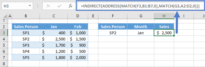
Let’s walk through the formula:

AutoMacro | Excel Automation Made Easy | Free Trial

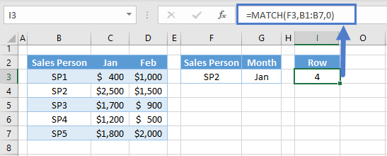
Row Coordinate

In this formula, we must determine the row coordinate of the cell itself unlike the INDEX and OFFSET formulas where we used relative coordinates.

=MATCH(F3,B1:B7,0)

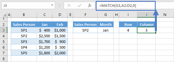
Column Coordinate

Next, we also need to determine the column coordinate of the cell.

=MATCH(G3,A2:D2,0)

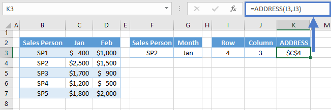
ADDRESS Function

Next, we use the row and column coordinates to return a cell reference in text format using the ADDRESS Function. By default, the text cell reference will be in absolute form (e.g., $C$4).

=ADDRESS(I3,J3)

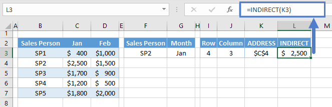
INDIRECT Function

Last, we convert the text cell reference into a real cell reference by using the INDIRECT Function.

=INDIRECT(K3)

Note: INDIRECT Function is a volatile function, which means it will always recalculate whenever the sheet recalculates. Depending on the scenario, this can affect the speed of your sheet.

Combining all the functions together yields our original formula:

=INDIRECT(ADDRESS(MATCH(F3,B1:B7,0),MATCH(G3,A2:D2,0)))

AutoMacro | Excel Automation Made Easy | Free Trial

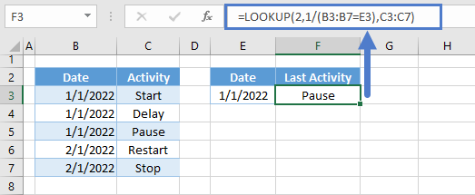
6. The LOOKUP Function: Last Match

If there are duplicate entries within the lookup array, getting the last match is difficult for the VLOOKUP Function. The XLOOKUP Function is the best solution, but if that’s not an option, the LOOKUP Function is the best alternative.

=LOOKUP(2,1/(B3:B7=E3),C3:C7)

Let’s walk through the formula:

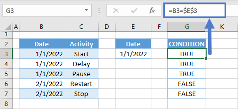
Lookup Condition

First, let’s check the values from the lookup column (e.g., B3:B7) against the lookup value (e.g., E3).

=B3=$E$3

Reciprocal of Boolean Values

Next, we take the reciprocal of the Boolean values, where TRUE is 1 and FALSE is 0.

=1/G3

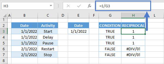
The reciprocal array is used as the lookup array for the LOOKUP Function, which ignores errors. Therefore, we technically have an array of 1s.

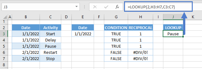
LOOKUP Function

The LOOKUP Function can only do an approximate match with the assumption that the data is sorted in ascending order, which means that the LOOKUP Function will find the largest value from the lookup array that is less than or equal to the lookup value.

We used 2 as the lookup value to take advantage of the approximate match in the array of 1s. If there are duplicates, like the example, the position of the last instance is returned instead.

=LOOKUP(2,H3:H7,C3:C7)

Combining all formulas yields our original formula:

=LOOKUP(2,1/(B3:B7=E3),C3:C7)

AutoMacro | Excel Automation Made Easy | Free Trial

7. The FILTER Function: Look Up All Duplicates

If we want to look up all duplicates, newer versions of Excel offer a better alternative – the FILTER Function. It’s simple and doesn’t require a lot of steps like adding helper columns.

=FILTER(C3:C7,B3:B7=E2)

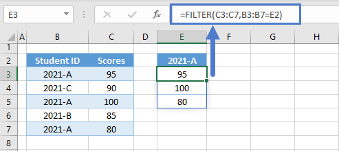
Note: The first argument is the array (e.g., C3:C7) that we want to filter, and the second argument is the filter criteria (e.g., B3:B7=E2).

8. FILTER-INDEX Formulas: Lookup nth Match

Instead of returning all duplicates, we can select the nth match using the FILTER-INDEX Formula. This is a more convenient alternative to the Unique ID – VLOOKUP Method (see VLOOKUP Duplicate Values article).

=INDEX(FILTER(C3:C7,B3:B7=E3),F3)

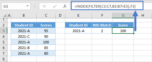
Let’s walk through the formula:

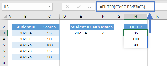
FILTER Function

First, let’s return all duplicates using the FILTER Function. We used the lookup array = lookup value as the filter condition.

=FILTER(C3:C7,B3:B7=E3)

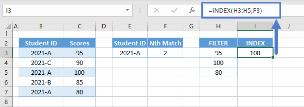
INDEX Function and Nth Match

Next, we return the nth match from the result of the FILTER Function using the INDEX Function.

=INDEX(H3:H5,F3)

Combining all functions yields our original formula:

=INDEX(FILTER(C3:C7,B3:B7=E3),F3)

AutoMacro | Excel Automation Made Easy | Free Trial

9. The SUMPRODUCT Function: Lookup Numbers

If we are only looking up numbers, we can use the SUMPRODUCT Function as an alternative for the VLOOKUP Function. One advantage of the SUMPRODUCT Function is the convenience of applying multiple criteria. For Excel users without access to new Array Formulas, you won’t need to use CTRL + SHIFT + ENTER to process the arrays. Let’s look at the example below:

=SUMPRODUCT((B3:B7=F3)*(C3:C7=G3)*D3:D7)

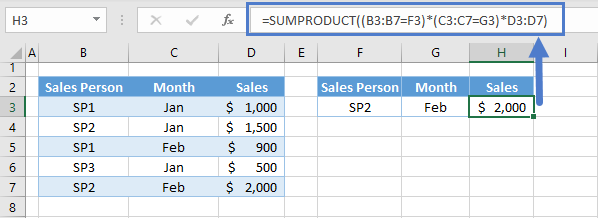
Let’s walk through the formula:

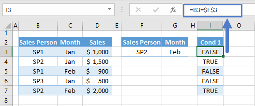
Condition 1

First, let’s apply the appropriate conditions to their corresponding columns. Here’s the first condition:

=B3=$E$3

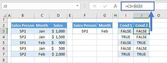
Condition 2

Here’s the second condition:

=C3=$G$3

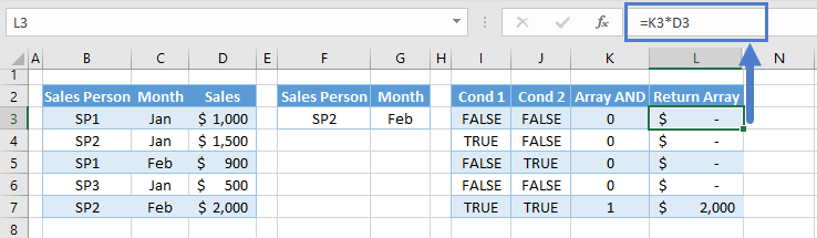
Array AND

Next, we check if both conditions are satisfied by multiplying the two Boolean arrays (TRUE = 1 and FALSE = 0).

=I3*J3

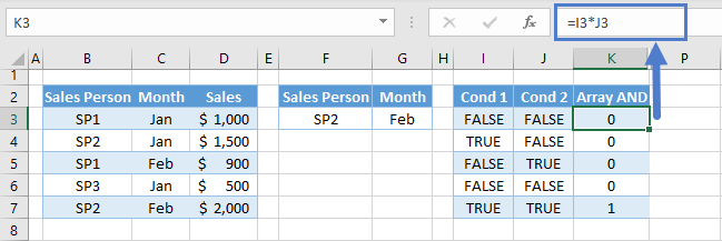
Note: Multiplying Boolean arrays are equivalent to the AND Function. If both conditions are satisfied, the result is 1. If one of the conditions is FALSE, then the product is 0.

AutoMacro | Excel Automation Made Easy | Free Trial

Return Array

If there are no duplicates, then the list will contain one value of 1 and the rest are 0s. We convert this array into the return array by multiplying the return array to it.

=K3*D3

SUMPRODUCT Function

The SUMPRODUCT Function performs an array multiplication and takes the sum of the product array. Since there’s only one value greater than 0 and the rest are 0, the sum will return the value that we are looking for.

=SUMPRODUCT(L3:L7)

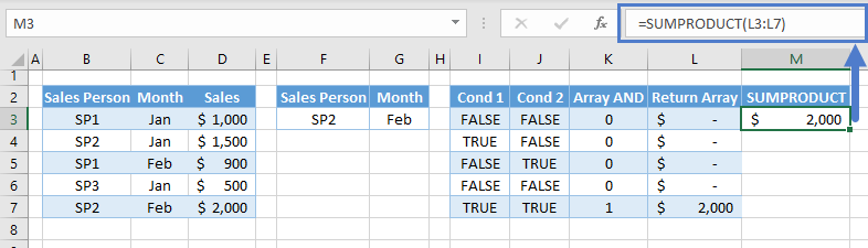
Note: We multiplied the arrays before the SUMPRODUCT Function to convert the Boolean arrays to numbers. The SUMPRODUCT Function only performs calculations with numbers and excludes other data types (e.g., Boolean, Strings).

Combining all formulas yields our original formula:

=SUMPRODUCT((B3:B7=F3)*(C3:C7=G3)*D3:D7)

10. The SUMIF Function: Lookup Numbers

Instead of the SUMPRODUCT Function, we can also use the SUMIFS Function to perform multiple criteria lookups on numbers. It’s simpler and more convenient to use compared to the SUMPRODUCT Function, but unlike the SUMPRODUCT Function, it can’t accept array inputs like array results from other functions. The sum_range and criteria_ranges are strictly ranges.

=SUMIFS(D3:D7,B3:B7,F3,C3:C7,G3)

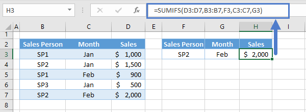
Note: The first argument is the sum_range, which is the array that will be summed. The succeeding arguments are pairs of criteria_ranges, where the criteria are checked against, and the criteria.

11. Google Sheets: The QUERY Function

Aside from the XLOOKUP Function, which does not exist in Google Sheets, all functions that were previously mentioned are available and work the same way in Google Sheets, but there’s a more powerful alternative that we can use in Google Sheets – the QUERY Function.

=QUERY(B3:C7,"SELECT C WHERE B='"&E3&"'")

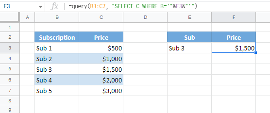
Note: The second argument of the QUERY Function is the query syntax (text format) that can help us perform data manipulations such as lookups, sorting, filtering and formatting.

Let’s walk through the formula:

AutoMacro | Excel Automation Made Easy | Free Trial

SELECT

The SELECT clause filters the column that we want to return (e.g., Column C).

=QUERY(B3:C7,"SELECT C")

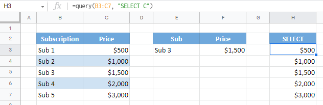
Note: If we remove the SELECT clause, all columns will be returned instead.

WHERE

The WHERE clause filters the row. Since the lookup value is a text, we need to enclose it with single quotations.

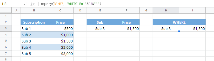
Combining both clauses yields our original formula:

=QUERY(B3:C7,"SELECT C WHERE B='"&E3&"'")