Excel COUNTBLANK Function Examples – Excel & Google Sheets

Written by

Editorial Team

Reviewed by

Steve Rynearson

Last updated on November 9, 2023

This tutorial demonstrates how to use the COUNTBLANK Function in Excel.

COUNTBLANK MAIN Function

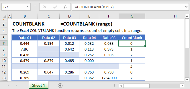
What is the COUNTBLANK Function?

The Excel COUNTBLANK Function returns the number of empty cells within a given range.

How to Use the COUNTBLANK Function

You use the Excel COUNTBLANK Function like this:

=COUNTBLANK(B3:B11)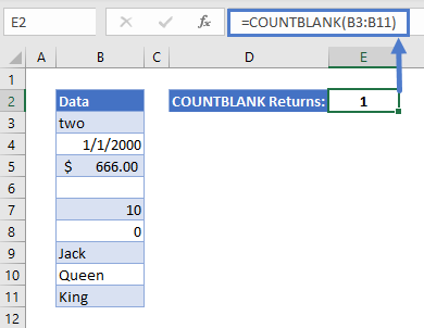

How to Use COUNTBLANK

In this example, COUNTBLANK returns 1, since the range B3:B11 has one blank cell in it (B6).

What Is a Blank Cell?

COUNTBLANK counts the following cells as blank:

Completely empty cells
Cells with a formula that returns an empty string, for example: =””

COUNTBLANK does NOT count:

Cells that only contain spaces (this is treated as any other text string)
Cells containing 0
Cells containing FALSE

The example below shows each of the above cases in sequence:

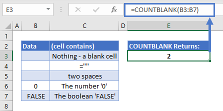
As you can see, COUNTBLANK returns 2 – the top two cells. It ignores the lower three cells.

Using COUNTBLANK to Highlight rows with Missing Data

With Excel’s conditional formatting feature, you can apply formatting to cells within a range based on criteria that you define.

You can combine conditional formatting with COUNTBLANK to automatically highlight rows with blank cells in them. This is very handy for spotting missing data that might throw off your calculations.

Take a look at the following data:

Highlight A

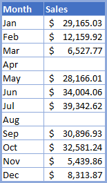
As you can see, someone’s forgotten to put the sales figures in for April and August. Easy to spot on a small table like this – but on a larger spreadsheet, an oversight like this could go unnoticed.

Here’s how to highlight it:

Select your data range
Go to the Home tab, click “Conditional Formatting” from the “Styles” menu, then click “New Rule”
Click “Use a formula to determine which cells to format”
Enter the following formula in the box that appears:

=COUNTBLANK($B3:$C3)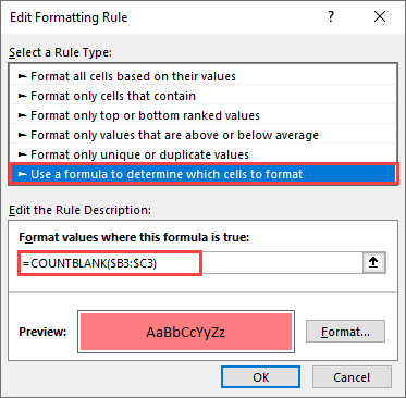

Conditional Format

Just make the range the first row of your data, and put a dollar sign before both cell references. This will make Excel apply the formatting to the entire row.

Click “Format”, and then choose whatever formatting you like. I’m just going to go for a red fill color.
Click “OK”, and “OK” again.

Here’s the result:

Highlight B

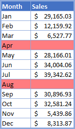
Now we can which rows contain blank cells at a glance.

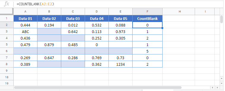
COUNTBLANK in Google Sheets

The COUNTBLANK Function works exactly the same in Google Sheets as in Excel:

COUNTBLANK Google Function