SUMPRODUCT – How Does it Work? Arrays, Criteria – Excel & Google Sheets
Written by
Reviewed by
Download the example workbook
This Tutorial demonstrates how to use the Excel SUMPRODUCT Function in Excel and Google Sheets.
SUMPRODUCT Function Overview
The SUMPRODUCT Function Multiplies arrays of numbers and sums the resultant array.
It is one of the more powerful functions within Excel. It’s name, might lead you to believe it’s only meant for basic math calculations (weighted average), but it can be used for so much more.
Basic Math
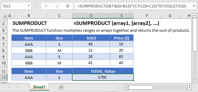
Let’s look at a basic example of SUMPRODUCT, using it to calculate total sales.
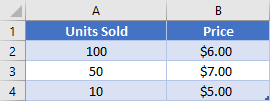
We have our table of products, and we want to calculate the total sales. You be tempted to just add a new column, take the quantity sold * price and then sum up the new column. Instead, however, you can simply use the SUMPRODUCT Function. Let’s walk through the formula:
=SUMPRODUCT(A2:A4,B2:B4)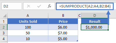 The function will load the ranges of numbers into arrays, multiple them against each other, and then sum the results:
=SUMPRODUCT({100, 50, 10}, {6, 7, 5})
=SUMPRODUCT({100 * 6, 50 * 7, 10 * 5})
=SUMPRODUCT({600, 350, 50}
=1000
The SUMPRODUCT Function was able to multiply all the numbers for us AND do the summation.
Weighted Average
Another case where it’s helpful to use SUMPRODUCT is when you need to calculate a weighted average. This most often occurs when dealing with schoolwork, so let’s consider the following table.
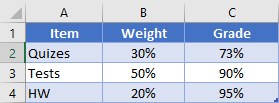
We can see how much the quizzes, tests, and homework are worth toward the overall grade, as well as what the current average is for each particular item. We can calculate the overall grade then by writing
=SUMPRODUCT(B2:B4, C2:C4)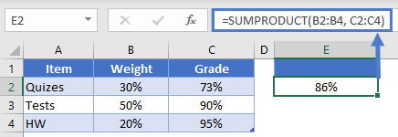
Our function again multiplies each item in the arrays before summing the total. This works out like so
=SUMPRODUCT({30%, 50%, 20%}, {73%, 90%, 95%})
=SUMPRODUCT({22%, 45%, 19%})
=86%
Multiple Columns
Another place we might use SUMPRODUCT is with even more columns that need to all be multiplied against each other. Let’s look at an example where we need to calculate volume in pieces of lumber.
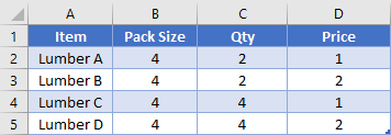
Rather than creating a helper column to calculate the total sale for each row, we can do this with a single formula. Our formula will be
=SUMPRODUCT(B2:B5, C2:C5, D2:D5)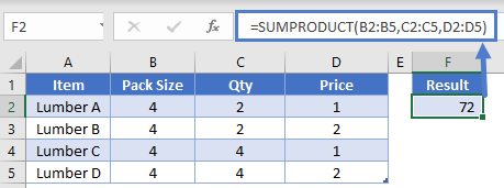 Each arrays’ first items will multiply against each other (e.g., 4 * 2 * 1 = 8). Then, the 2nd (4 * 2 * 2 = 16), and 3rd, etc. Overall, this will product the array of products that look like {8, 16, 16, 32). Then the total volume would be the sum of that array, 72.
Arrays
SUMPRODUCT requires inputs of arrays.
So first, what do we mean by “array”? An array is simple a group of items (ex. numbers) arranged in a specific order, just like a range of cells. So, if you had the numbers 1, 2, 3 in cells A1:A3, Excel would read this as array {1,2,3}. In fact, you can enter {1,2,3} directly into Excel formulas and it will recognize the array.
We’ll talk more about arrays below.
One criteria
Okay, let’s add another layer of complexity. We’ve seen that SUMPRODUCT can handle arrays of numbers, but what about if we want to check for criteria? Well, you can also create arrays for Boolean values (Boolean Values are values that are TRUE or FALSE).
For instance, take a basic array {1, 2, 3}. Let’s create a corresponding array that indicates if each number is greater than 1. This array would look like {FALSE, TRUE, TRUE}.
This is extremely helpful in formulas, because we can easily convert TRUE / FALSE into 1 / 0. Let’s look at an example.
Using the below table, we want to calculate “How many units sold were Red?”
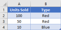
We can do so, with this formula:
=SUMPRODUCT(A2:A4, --(B2:B4="Red"))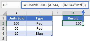
“Hold on! What’s with the double minus symbol there?” you say. Remember how I said we could convert from True/False into 1/0? We do this by forcing the computer to do a mathematical operation. In this case, we’re saying “take the negative value, and then take the negative again”. Writing that out, our array is going to change like this:
{True, True, False}
{-1, -1, 0}
{1, 1, 0}
So, back to the full SUMPRODUCT formula, it’s going to load in our arrays and then multiply, like this
=SUMPRODUCT({100, 50, 10}, {1, 1, 0})
=SUMPRODUCT({100, 50, 0})
=150
Note how the 3rd item became a 0, because anything multiplied by 0 becomes zero.
Multiple criteria
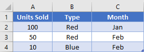
We can load up to 255 arrays into our function, so we can certainly load in more criteria. Let’s look at this bigger table where we’ve added the Month sold.
If we want to know how many items sold were red and were in the month of February, we could write our formula like
=SUMPRODUCT(A2:A4, --(B2:B4="Red"), --(C2:C4="Feb"))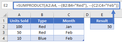 The computer would then evaluate our arrays and multiply across. We’ve already covered how True/False arrays get changed into 1/0, so I’m going to skip that step for now.
=SUMPRODUCT({100, 50, 10}, {1, 1, 0}, {0, 1, 1})
=SUMPRODUCT({0, 50, 0})
=50
We only had one row in our example that matched all criteria, but with real data, you might have had multiple rows that you needed added together.
Complex criteria
Okay, up to this point, you might not be impressed because all of our examples could have been done using other functions like SUMIF or COUNTIF. Now we’re going to do something those other functions can’t do. Previously, our Month column had the actual names of months. What if instead it had dates?

We can’t do a SUMIF now, because SUMIF can’t handle the criteria we need. SUMPRODUCT though can handle us manipulating the array though, and doing a deeper test. We’ve already been manipulating arrays when we’ve translated the True/False into 1/0. We’re going to manipulate this array with the MONTH function. Here’s the full formula we’re going to use
=SUMPRODUCT(A2:A4, --(B2:B4="Red"), --(MONTH(C2:C4)=2))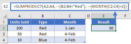 Let’s look at the 3rd array more closely. First, our formula is going to extract the month number from each date in C2:C4. This will give us {1, 2, 2}. Next, we check if that value equals 2. Now our array looks like {False, True, True}. We do the double minus again, and we have {0, 1, 1}. We’re now back in a similar spot we had in Example 3, and our formula will be able to tell us that there were 50 units sold in February that were red.
Double minus vs. multiplying
If you’ve seen the SUMPRODUCT function in use before, you might have seen a slightly different notation. Rather than using a double minus, you can write
=SUMPRODUCT(A2:A4*(B2:B4="Red")*(MONTH(C2:C4)=2))The formula is still going to work the same way, we’re just manually telling the computer that we want to multiply the arrays. SUMPRODUCT was going to do this anyway, so there’s no change there in how the math works. Performing the math operation converts our True/False into 1/0 the same. So, why the difference?
Most of the time, it doesn’t matter too much, and it comes down to user preference. There is at least one case though where multiplying is needed.
When you use SUMPRODUCT, the computer expects all the arguments (array1, array2, etc.) to be the same size. This means they have the same number of rows or columns. However, you can do what’s know as a two dimensional array calculation with SUMPRODUCT that we’ll see in next example. When you do that, the arrays are different sizes, so we need to bypass that “all the same size” check.
Two dimensions
All the previous examples had our arrays going in the same direction. SUMPRODUCT can handle things going in two directions, as we’ll see in next table.
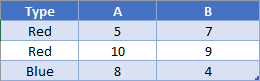
Here’s our table of units sold, but the data is rearranged where categories are going across the top. If we want to find out how many items were Red and in category A, we can write
=SUMPRODUCT((A2:A4="Red")*(B1:C1="A")*B2:C4)What is going on here?? It turns out that we’re going to be multiplying in two different directions. Visualizing this is harder to do with just a written sentence, so we’ve got a few images to help us out. First, our row criteria (is it Red?) is going to multiply across each row in the array.
=SUMPRODUCT((A2:A4="RED")*B2:C4)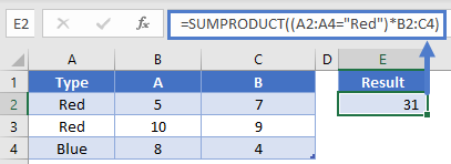
Next, the column criteria (is it category A?) is going to multiply down each column
=SUMPRODUCT((A2:A4="Red")*(B1:C1="A")*B2:C4)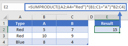
After both of those criteria have done their work, the only non-zeros left are the 5 and 10. SUMPRODUCT will then give us the grand total of 15 as our answer.
Remember how we talked about the arrays needing to be the same size unless you’re doing two dimensions? That was partially correct. Looks again at the arrays we used in our formula. The height of two of our arrays is the same, and the width of two of our arrays are the same. So, you still need to make sure that things are going to line up correctly, but you can do it in different dimensions.
Two dimensions and complex
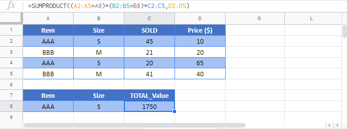
Many times we’re presented with data that isn’t in the best layout suitable for our formulas. We could try to manually rearrange it, or we can be smarter with our formulas. Let’s consider the following table.
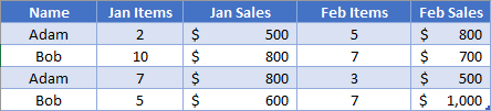
Here we have the data for our items and sales mixed together for each month. How would we go about finding out how many items Bob has sold for the entire year?
To do this, we’ll use two additional functions: SEARCH and ISNUMBER. The SEARCH function is going to let us look for our keyword “items” within the header cells. The output from this function is going to either by a number or an error (if the keyword isn’t found). Then, we’ll use the ISNUMBER to convert that output into our Boolean values. Our formula is going to look like below.
You should be pretty familiar with the first array by now. It’s going to create an output like {0, 1, 0, 1}. The next criteria array we just talked about. It’s going to create a number for all the cells with “Items” in them, and an error for the others {5, #N/A!, 5, #N/A!}. The ISNUMBER then converts this to Boolean {True, False, True, False}. Then when we multiply, it’s only going to keep values from the first and third column. After all the arrays multiply against each other, the only non-zero numbers we’ll have are the ones highlighted here:
=SUMPRODUCT((A2:A5="Bob")*(ISNUMBER(SEARCH("Items",B1:E1))*B2:E5))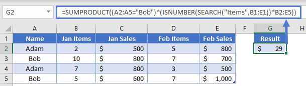
The SUMPRODUCT will then add those all up, and we get our final result of 29.
SUMPRODUCT Or
Many situations arise where we’d like to be able to sum up values if our criteria column has one value OR another value. You can accomplish this in SUMPRODUCT by adding two criteria arrays against each other.
In this example, we want to add up units sold for both Red and Blue.
Our formula will look like this
=SUMPRODUCT(A2:A7, (B2:B7="Red")+(B2:B7="Blue"))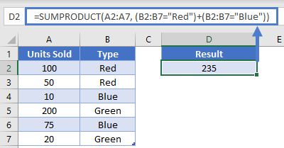 Let’s look at the Red criteria array. It will product an array that looks like this: {1, 1, 0, 0, 0, 0}. The Blue criteria array will look like {0, 0, 1, 0, 1, 0}. When you add them together, the new array will look like {1, 1, 1, 0, 1, 0}. We can see how the two arrays have blended together into a single criteria array. The function will then multiply that by our first array, and we’ll get {100, 50, 10, 0, 75, 0}. Notice that the values for Green have been zeroed out. The final step of the SUMPRODUCT is adding all the numbers together to reach our solution of 235.
One word of caution here. Be careful about when the criteria arrays are not mutually exclusive. In our example, the values in column B could be either Red or Blue, but we knew it could never be both. Consider if we’d written this formula:
=SUMPRODUCT(A2:A7, (A2:A7>=50)+(B2:B7="Blue"))Our intent is to find Blue items that were sold or were in a quantity more than 50. However, these conditions are not exclusive, as a single row could be both over 50 in column A and be Blue. This would result in the first criteria array look like {1, 1, 0, 1, 1, 0}, the second criteria array being {0, 0, 1, 0, 1, 0}. Adding them together produced {1, 1, 1, 1, 2, 0}. Do you see how we have a 2 in there now? If left alone, the SUMPRODUCT would end up doubling the value in that row, changing the 75 to a 150, and we’d get the wrong result. To correct for this, we place an outer criteria check on our array, like so:
=SUMPRODUCT(A2:A7, --((A2:A7>=50)+(B2:B7="Blue")>0))Now, after the two inner criteria arrays have been added together, we’ll check if the result is greater than 0. This gets rid of the 2 we had before, and instead we’ll have an array like {1, 1, 1, 1, 1, 0} which will produce the correct result.
SUMPRODUCT Exact
Most functions in Excel are not case-sensitive, but sometimes we need to be able to do a lookup with case sensitivity in mind. When the desired result is numerical, we can accomplish this by using the EXACT Function inside the SUMPRODUCT function. Consider the following table:
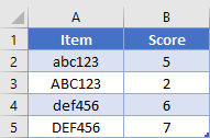
We want to find the score for Item “ABC123”. Normally, the EXACT function will compare two items and return a Boolean output stating whether the two items are exactly the same. However, since we’re inside of a SUMPRODUCT, our computer will know that we are dealing with arrays and will be able to compare one item with each item in an array. Our formula will look like this
=SUMPRODUCT(--EXACT("ABC123", A2:A5), B2:B5)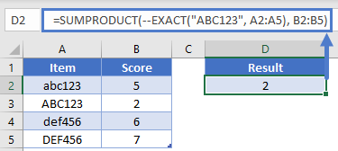
The EXACT function will then check each item in A2:A5 to see if it matches value and case. This will product an array that looks like {0, 1, 0, 0}. When multiplied against B2:B5, the array becomes {0, 2, 0, 0}. After the final summation, we get our solution of 2.
SUMPRODUCT in Google Sheets
The SUMPRODUCT Function works exactly the same in Google Sheets as in Excel:
SUMPRODUCT Examples in VBA
You can also use the SUMPRODUCT function in VBA. Type: application.worksheetfunction.sumproduct(array1,array2,array3)
Executing the following VBA statements
Range("B10") = Application.WorksheetFunction.SumProduct(Range("A2:A7"), Range("B2:B7"))will produce the following results
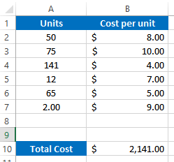
For the function arguments (array1, etc.), you can either enter them directly into the function, or define variables to use instead.

