UNIQUE Function Examples – Excel & Google Sheets
Written by
Reviewed by
This tutorial demonstrates how to use the UNIQUE Function in Excel to return a list of unique values in a list or range.
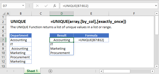
How to use the UNIQUE Function
The UNIQUE function is used to extract unique items from a list.
For example, if we wanted to return a list of unique departments from our list in A2:A7, we enter the following formula in D2:
=UNIQUE(A2:A7)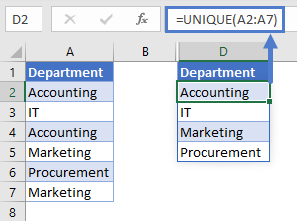
It can also be used to extract items that only appear once in a list.
For example, if we wanted to return a list of departments that appear only once in our list in A2:A7, we enter the following formula in D2:
=UNIQUE(A2:A7,FALSE,TRUE)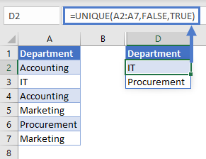
Unique Items from a List
To extract a list of unique Employees we enter the following formula in D2:
=UNIQUE(A2:A7)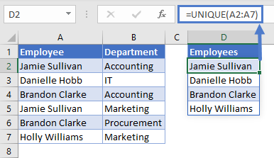
If our list was across columns, we would enter the following formula in C4:
=UNIQUE(C2:H2,TRUE)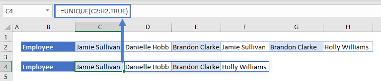
We set the 2nd argument [by col] to ‘TRUE’ to enable the formula to compare the columns against each other.
Return Items Only Appearing Once
To extract a list of Employees that appear only once, we enter the following formula in D2:
=UNIQUE(A2:A7,FALSE,TRUE)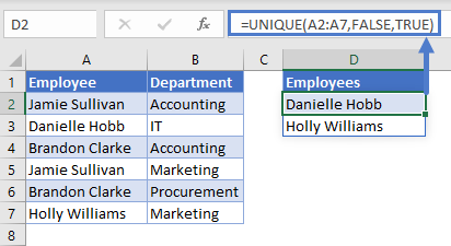
We set the 3rd argument [exactly_once] to ‘TRUE’ to extract items that only appear once in our list.
Return Items in Alphabetical Order
To extract a list of unique Employees and sort their names in alphabetical order, we use the UNIQUE Function together with the SORT Function. We enter the following formula in D2:
=SORT(UNIQUE(A2:A7))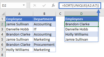
Ignore Blanks
If a blank value exists in the list (selected range) it will be returned as a ‘0’.
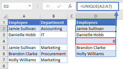
To ignore blanks in a list, we use the UNIQUE Function together with the FILTER Function.
We enter the following formula in D2:
=UNIQUE(FILTER(A2:A7,A2:A7<>""))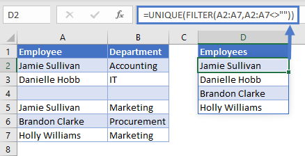
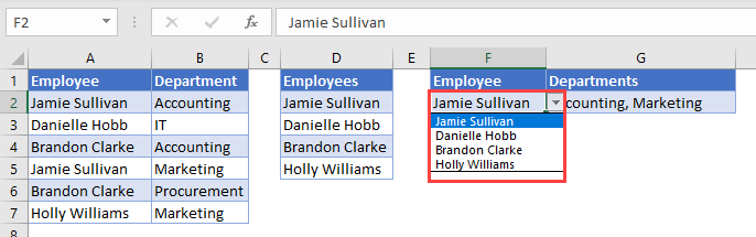
Dynamic Data Validation Drop-Down List
You can use the list generated by the UNIQUE function to create a data validation drop-down list.
In this example we’d like to create a drop-down where a user can select an Employee and view the department they work in.
To first step is to create the list that the drop-down will use, we enter the following formula in D2:
=UNIQUE(A2:A7)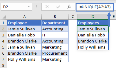
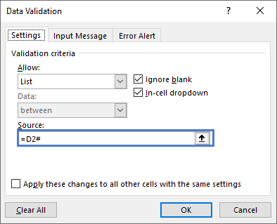
The next step is to add Data Validation to cell F2. We add the source of our Data Validation list as ‘D2#’ . We use the ‘#’ sign after the cell reference ‘D2’ so that we can refer to the whole list that the UNIQUE Function generates.
Issues
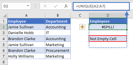
#SPILL!
This error occurs when there is a value in the Spill Range i.e. the range where the UNIQUE Functions lists the unique items.
To correct this error, clear the range that Excel highlights.
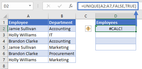
#CALC!
This error occurs when the UNIQUE Function is unable to extract a list of unique or distinct items. In the example below, we’d like to extract a list of Employees that appear only once but because all Employees appear twice the #CALC! error is returned.
UNIQUE Tips & Tricks
- Ensure that the cells below the input cell are blank to avoid the Spill Error, learn more about the Spill Error ‘here’ — add link to Intro to DAFs.
- UNIQUE can be used with other Excel Functions such as the FILTER Function and SORT Function to create more versatile formulas.
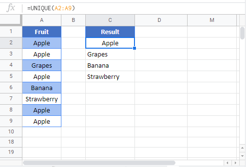
UNIQUE in Google Sheets
The UNIQUE Function works exactly the same in Google Sheets as in Excel: