Pivot Table – Count Unique Values in Excel and Google Sheets

This tutorial demonstrates how to count unique values with a pivot table in Excel and Google Sheets.

 

 

Count Distinct Values in a Pivot Table

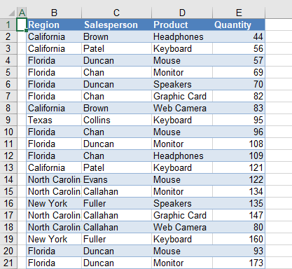
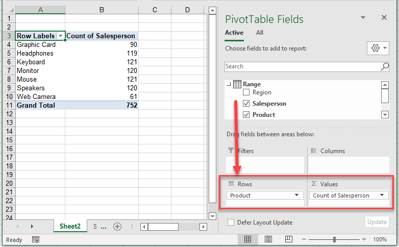
Consider the following table of data. Say you want to count the number of salespeople. Since each person has multiple records in the dataset, you need to make sure your count doesn’t include duplicates.

 

 

1. In the Ribbon, go to Insert > PivotTable.

 

 

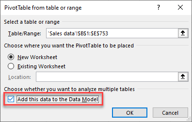
2. Make sure that Add this data to the Data Model is checked, and then click OK.

 

 

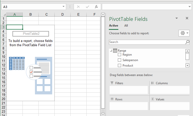
3. Now drag the Product field down to the Rows area, and the Salesperson field down to the Values area.

 

 

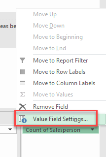
4. In the drop down next to the count of the Salesperson field, choose Value Field Settings.

 

 

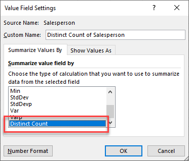
5. From the Summarize value field by list, choose Distinct Count, and then click OK.

 

 

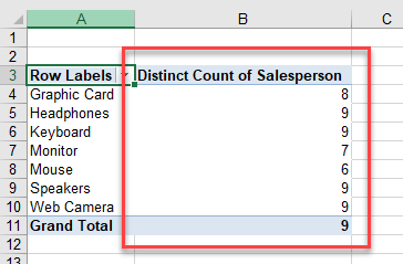
The data is changed to show how many salespeople sold a particular product.

Tip: Try using some shortcuts when you’re working with pivot tables.

Count Unique Values in Google Sheets Pivot Table

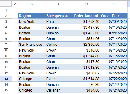
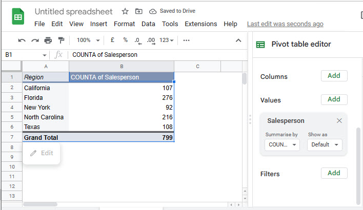
Counting unique values can done in Google Sheets with a pivot table too, but it’s done a bit differently. Say, again, that you want to count the number of salespeople in the dataset (partially) pictured below.

 

 

1. First, create a pivot table, adding Region as a Row and the Salesperson as a Value. As the Salesperson field isn’t made up of numeric figures, the pivot table editor automatically adds a COUNTA summary for that field.

 

 

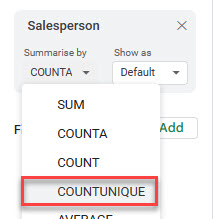
2. In the Summarize by drop down, change the function from COUNTA to COUNTUNIQUE.

 

 

Now the data only shows how many salespeople are in each specific region.

 

 

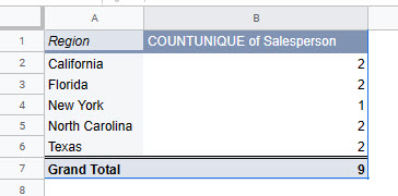
Note: Although it doesn’t apply to this example, the Grand Total may not equal the sum of the row values. If one salesperson worked in both California and Florida, for example, they would be counted once in Row 2, once in Row 3, and once in Row 7; the sum of B2:B6 would be 10, but the grand total would still be 9.