How to Create a Slider Bar (Scroll Bar) in Excel

This tutorial demonstrates how to create a slider bar in Excel.

Create a Scroll Bar

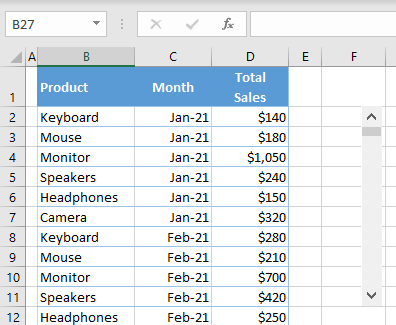
The built-in scroll bar in Excel lets you scroll the whole worksheet, but you can also create your own scroll bar that only applies to a specific range of cells. This can be useful when you have large sets of data and want to display only a fixed number of rows at a time. Say you have the following table of sales data.

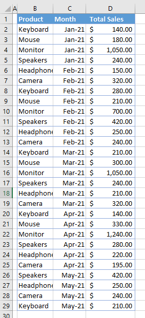
From this dataset, you can create a second range, with the same data, that displays only ten rows at a time and updates which rows are displayed as you scroll up or down.

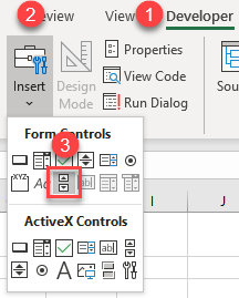
1. In the Ribbon, go to Developer > Insert > Scroll Bar (Form Control).
   Note: Add the Developer tab to the Ribbon if you don’t already see it.

2. Click in the worksheet where you want to insert a scroll bar.

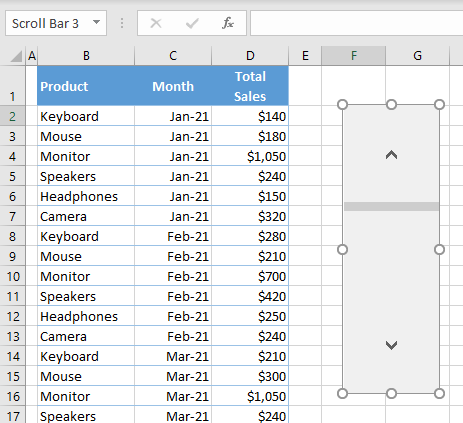
3. A scroll bar is added to the worksheet, but it’s not in a useful shape or size. Resize it to fit ten rows in Column F.

4. Right-click the scaled scroll bar and choose Format Control…

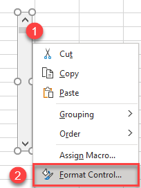
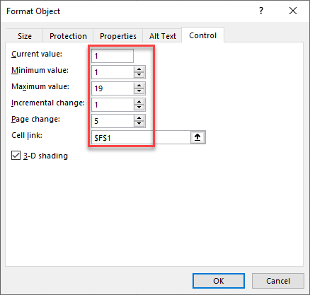
5. In the Format Object window, set the values for the scroll bar.

• The Current Value is what the scroll bar will be initially set to in your worksheet while the Minimum value is the lowest value that the scroll bar can go to. Set 1 for both the Current value and Minimum value.
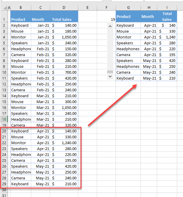
• The Maximum values is the highest value that the scroll bar can go up to. Set 19 for the Maximum value. This lets the scrollable list show the data through Row 29 in the Excel sheet. (Scroll from Row 2 to Row 29 as the list will show 10 records at a time; when the scroll bar value is 19, Rows 20–29 are shown.)
• As you click down (or up) the scroll bar, it moves by a set incremental value. Set the Incremental change to 1 so that with each click, the value moves up or down by 1.
• If you click in the scroll bar (and not on the up or down arrow), the scroll bar value will move by a set amount, referred to as the page change. Set the Page change to 5. This means that the scroll bar jumps up or down 5 rows at a time.
• Set the Cell link to F1. As you scroll up or down, the scroll bar value is shown in the linked cell. This is also used by the formula below to show the correct data when the scroll bar is clicked.

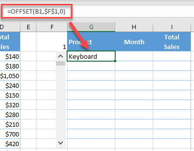
6. Now format the header of the new table (G1:I1), just like in the source dataset. In cell G2, enter the formula:

=OFFSET(B1,$F$1,0)

The OFFSET Function outputs a value that is one row under B1 (because the value in F1 is 1) as the user scrolls. For example, the value in F1 is 2, and the formula returns the value two rows under B1, etc.

7. Now copy the formula to Columns H and I, and through Row 11 in order to populate all data from the initial dataset.

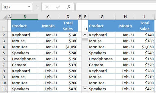
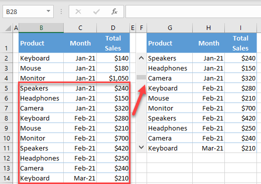
8. As you can see, the scroll bar is in the initial position (1 in F1) and Rows 2–11 (from the source) are displayed. Scroll the slider down two times to display Rows 4–13.

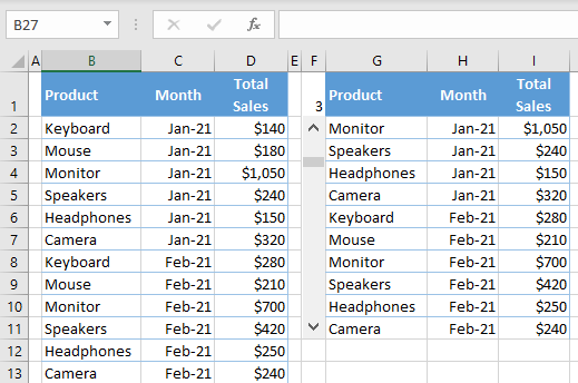
If you scroll down to the bottom of the scroll bar, the value in F1 will be 19 and Rows 20–29 are shown.