Freeze / Unfreeze Panes – Excel & Google Sheets **Updated 2023**

This tutorial demonstrates how to freeze and unfreeze panes in Excel and Google Sheets.

 

If you have a large worksheet, it is sometimes useful to always be able to see a few specific columns on the left side of your screen even when you scroll to the right; and a top row, or few rows when you scroll down your worksheet. Making these columns and or rows always visible is known as freezing panes.

There are three options available for freezing panes.

Freeze Panes

This option enables you to freeze more than one row or column. Depending on where you mouse pointer is placed, the rows above, and the columns to the left are always visible.

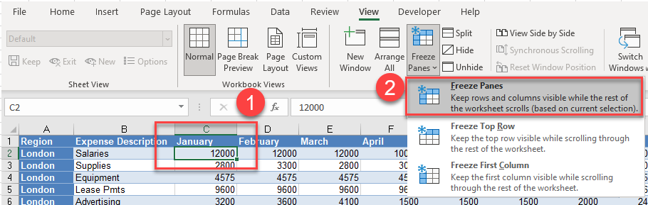
1. Select where you wish the freeze to take place.
2. In the Ribbon, go to View > Windows > Freeze Panes > Freeze Panes. (The shortcut for this action is ALT > W > F > F.)

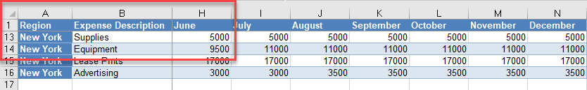
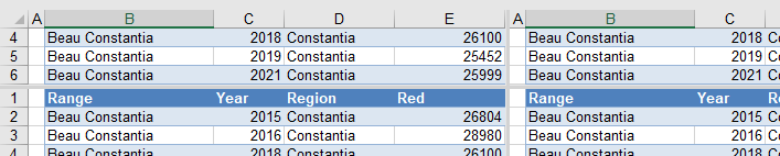
Now, when you scroll down or across, you always have the first row and the two left columns visible.

Split Panes

In addition to the Freeze Panes command, the Windows group in the View tab on the Ribbon also offers a Split feature. This feature actually enables you to split your screen into four separate portions, each of which you can scroll independently.

1. Select the cell at the position where you want to split the screen horizontally and vertically. (The picture below shows the result of splitting, rather than freezing, at E7.)
2. In the Ribbon, go to View > Split. (The shortcut for this action is ALT > W > S.)

Freeze Top Row

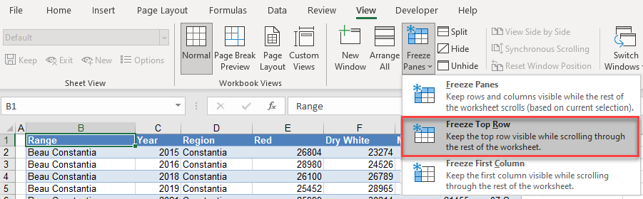
If the top row or rows of data in Excel contains headings and you have a lot of rows of data, you may want to make sure the top row remains in place as you scroll down your worksheet, so you can still see the headings contained in each column.

▸ In the Ribbon, go to View > Windows > Freeze Panes > Freeze Top Row. (The shortcut for this action is ALT > W > F > R.)

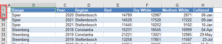
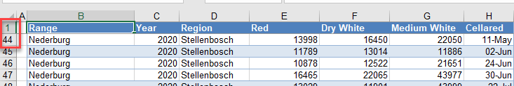
Now, when you scroll down, the top row remains in place.

Freeze First Column

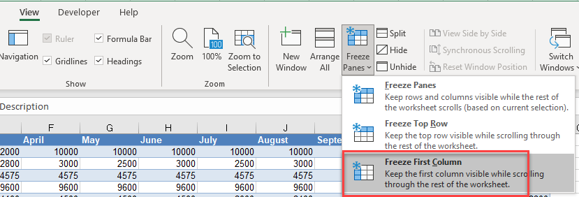
You can also lock the first column in place.

▸ In the Ribbon, go to View > Windows > Freeze Panes > Freeze First Column. (The shortcut for this action is ALT > W > F > C.)

Unfreeze Panes

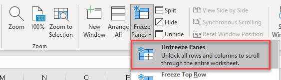
If any of your panes are already frozen, you can unfreeze panes and reset the view.

▸ In the Ribbon, go to View > Windows > Freeze Panes > Unfreeze Panes. (This shortcut is the same as the Freeze Panes one.)

Freeze / Unfreeze Panes in Google Sheets

The freeze functionality in Google Sheets works in a similar way.

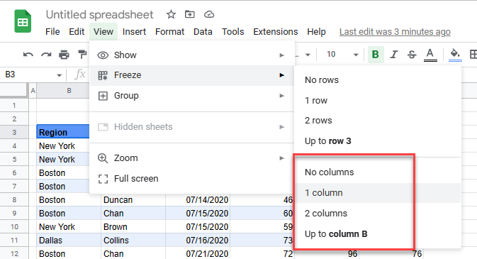
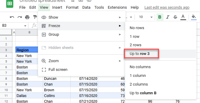
1. Select the row where you want the sheet frozen.
2. In the Menu, go to View > Freeze > Up to row 3 (with the number depending on the row selected).

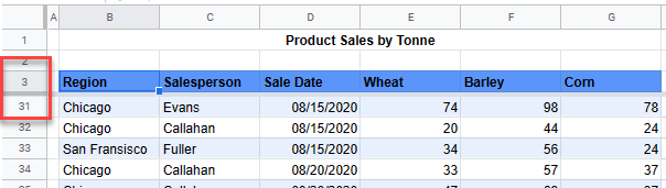
3. Scroll down the sheet with your mouse and notice that the first three rows are frozen in place.

You can freeze columns in a similar way.