How to Use Horizontal Filter in Excel & Google Sheets

This tutorial demonstrates how to apply a horizontal filter in Excel and Google Sheets.

 

 

Horizontal Filters

Filtering is used extensively in Excel to show and hide specific values in a dataset. Most often, you use a vertical filter, where the rows of the worksheet are filtered. A horizontal filter, where the columns of the worksheet are filtered, is not a built-in feature in Excel. You can, however, create a horizontal filter. Below are two ways.

Custom Views

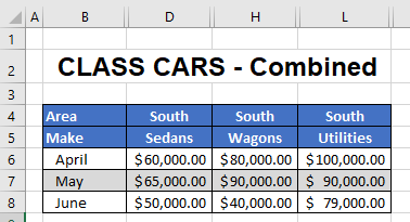
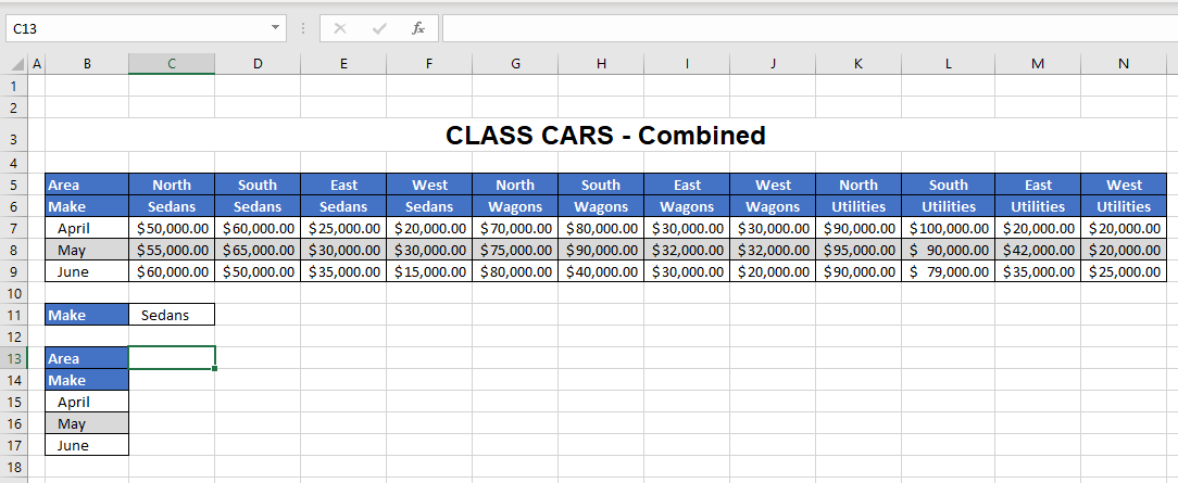
Consider the following worksheet:

 

 

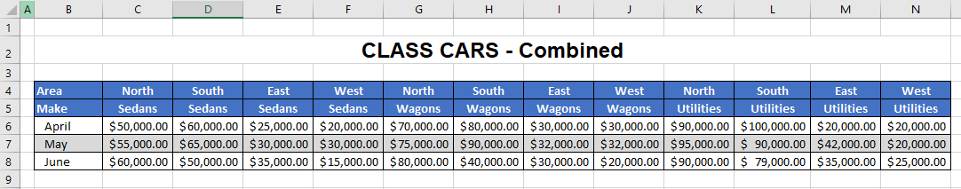
The data has been set out using columns across the worksheet instead of rows going down the worksheet. You may only wish to see one area at a time. For example, all the North data or all the South data OR you may wish to only see a certain make at a time e.g., Sedans, Wagons, or Utilities.

You can achieve this by creating custom views for the data.

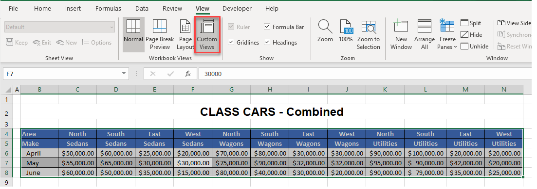
1. Select all data. You can do this quickly by clicking in the data and then pressing CTRL + A on the keyboard, or using the mouse to click and drag. Then, in the Ribbon, go to View > Workbook Views > Custom Views.

 

 

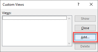
2. Click the Add… button to add a new view.

 

 

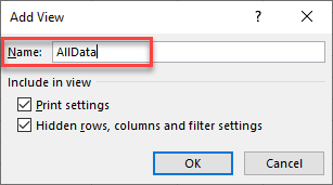
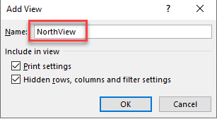
3. Type in the name of the view (in this case, AllData), then click OK.

 

 

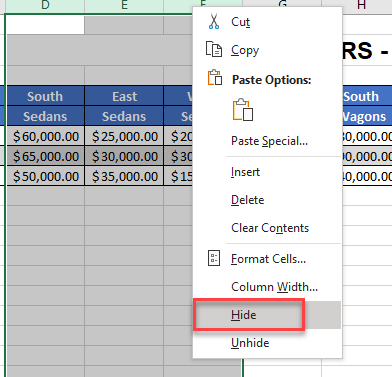
4. Now, in Excel, hide the columns to only show the data you need (for example, the North data).
   Right-click on the column header, and then click Hide.

 

 

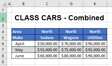
5. Repeat this until the only columns shown are what you want to see.

 

 

6. Click once again in the Ribbon, go to View > Workbook Views > Custom Views, and then click Add….
7. Type in the name of the view and click OK.

 

 

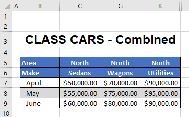
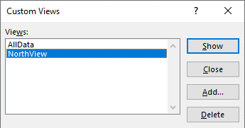
You now have two custom views in the list.

 

 

8. To show all the data again, click in the Ribbon, and then go to View > Workbook Views > Custom Views.
9. Select the view AllData, and then click Show. This, once again, shows all the columns in the worksheet.
10. Hide the columns for the next view (e.g., all the columns except the ones containing South data).

 

 

11. Create and name a view for this data. Then repeat the process for any other views.

 

 

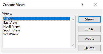
12. You can then use the Custom Views dialog box to toggle between the different views (filters) of data.
13. If you create a view that you no longer need, choose that view in the Custom Views dialog box, and then click Delete.

 

 

14. Click Yes to delete the custom view.

The FILTER Function

Excel 365 (and 2019) has the new FILTER Function available that enables you to filter horizontally in a worksheet.

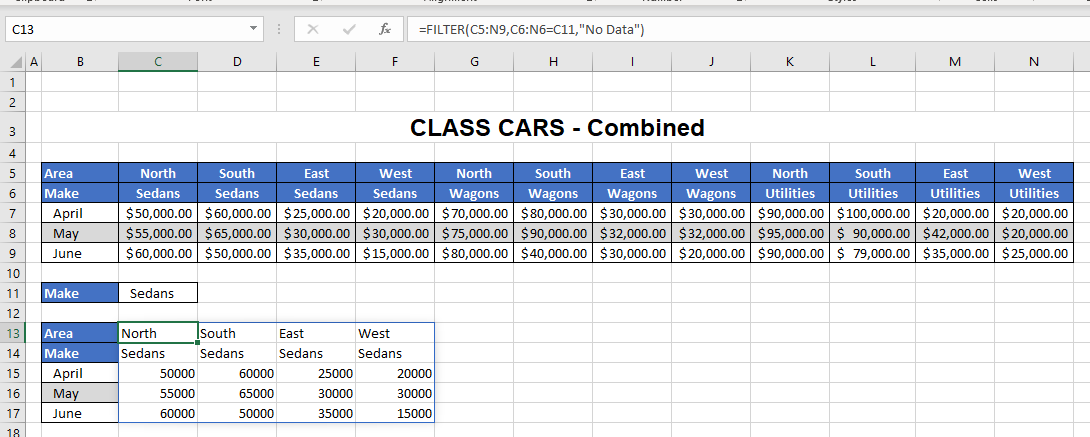
Consider the following worksheet.

 

 

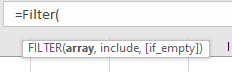
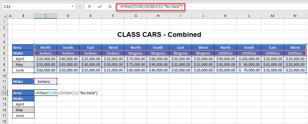
1. With the filter criteria in C11, type this formula into C13:

=FILTER(C5:N9,C6:N6=C11,"No Data")

The syntax of the formula is as follows:

 

 

• The array argument is the data you are including to filter on (C5:N9).
• The include argument is the row that contains the filter criteria (e.g., Make in Row 6) and must then match the filter criteria (i.e., C11).
• The [if empty] is optional and is the text that is returned if no data is found. You can make this any text within double quotation marks.

 

 

2. Once the formula is complete, press ENTER on the keyboard. This automatically populates a smaller table with filtered data.

 

 

3. You can change the criteria of the filter, for example, by changing the word Sedans to Wagons.

 

 

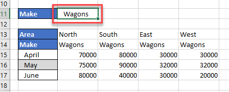
That updates the filtered data accordingly.

Horizontal Filters in Google Sheets

Google Sheets does not have the ability to set up views, but you can manually hide columns if needed. Sheets does, however, have a FILTER Function that can be used for horizontal filtering.

The syntax for the FILTER Function is:

=FILTER(array,criteria)

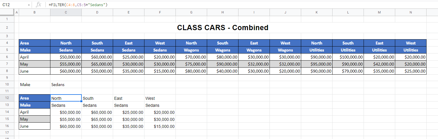
So, the filter for the worksheet as shown below would be:

=FILTER(C4:8, C5:5="Sedans")

• For the array, start in Column C, Row 4 to Row 8.
• For the criteria, look in Row 5 for the word Sedans.