Limit Decimal Places (Significant Figures) in Excel & Google Sheets
Written by
Reviewed by
This tutorial demonstrates how to limit decimal places (set the number of significant figures) for a value in Excel and Google Sheets.
You can either use the ROUND Function to limit decimal places in Excel, or you can use cell formatting to limit the number of decimal places displayed. The ROUND Function amends the original value; using cell formatting retains the exact original value.
ROUND Function
The ROUND Function is one of a few Excel functions that enables you to limit the number of decimal places in a cell.
- Select the cell to the right of the cell you wish to amend.
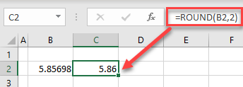
For this example, the original number is in cell B2.
- Type in the following formula:
=ROUND(B2,2)
Your data is rounded to 2 decimal places.
If there’s a column of data to round, copy the formula down.
You can also use the MROUND, ROUNDDOWN, FLOOR, ROUNDUP, CEILING, INT, and TRUNC Functions to round numerical data in Excel.
Limit Decimal Places
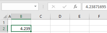
If you type a decimal number into a cell without any cell formatting (General format), Excel will display as many decimal places as the cell width allows for. For this example, consider a number with 8 decimal places, as shown below.
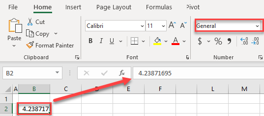
Column B has the standard width, so it displays 6 decimal places. Although you didn’t explicitly format the cell as a number, Excel recognizes is as a number and rounds it up (4.23871695 → 4.238717). Note that the stored value is exactly the same.
Theoretically, you can limit the number of decimal places by reducing the cell width, but it’s not a good option. For one, the width can sometimes change automatically if more data is entered into the column.
In the Ribbon
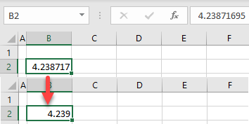
To decrease the number of decimal places, select the cell with a number (here, B2), and in the Ribbon, go to Home > Decrease Decimal.
One click decreases the number of decimal places by one.
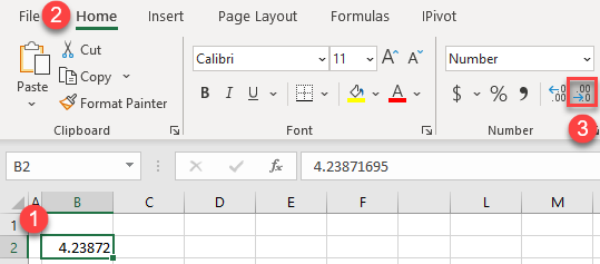
As shown in the picture above, the number of decimal places in cell B2 is decreased to 5. Also, the cell format automatically changes from General to Number.
Number Formatting
You can also limit decimal places using number formatting.
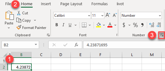
- Select the cell with a number (B2) and in the Ribbon, go to Home > Number Format.
- In the Format Cells window, enter the number of decimal places (for example, 3) and click OK. You can immediately see how the number will look in the Sample box.
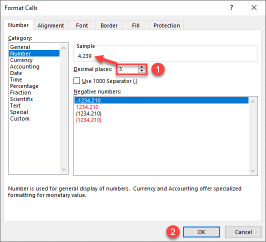
As a result, the number in cell B2 is rounded to 3 decimal places.
Note: If you format the cell as a number, Excel displays 2 decimal places by default.
See also…
Limit Decimal Places in Google Sheets
ROUND Function
The ROUND Functions works the same way in Google Sheets as it does in Excel.
Number Format
In Google Sheets, decimal numbers are also displayed depending on the column width. Unlike Excel, Google Sheets doesn’t automatically display rounded values. Therefore, if you reduce the column width, it won’t round the number, just cut off the extra decimal places.
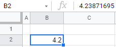
When you format the cell as a number, it’s rounded to 2 decimal places. Follow these steps to reduce the number of displayed decimal places to one:
- First format the cell as a number. Select the cell (B2) and in the Menu, go to Format > Number > Number.
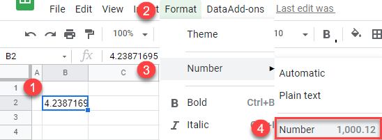
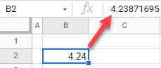
Now cell B2 is formatted as a number with – by default – 2 decimal places.
- Now you can limit the decimal places. Select the number cell and in the Menu, go to Format > Number > More Formats > Custom number format.
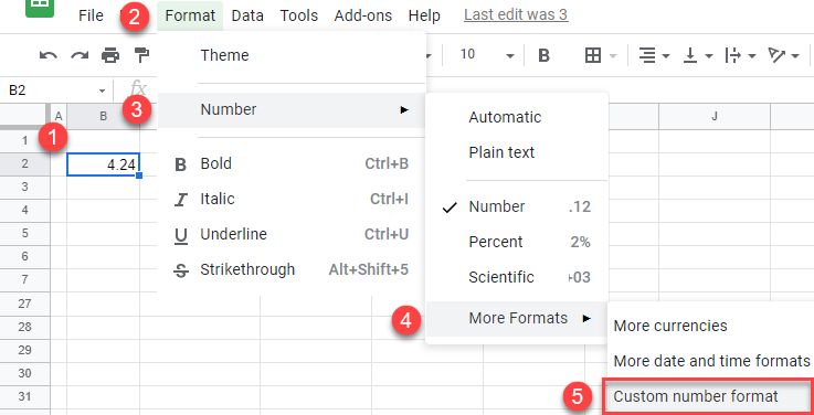
- In the Custom number formats window, enter #,##0.0 and click Apply. Zeros after the decimal point represent the number of decimal places that will be displayed.
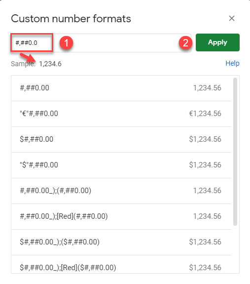
Finally, the number in cell B2, as displayed, is limited to 1 decimal place.