How to Add / Remove Strikethrough in Excel & Google Sheets
Written by
Reviewed by
This tutorial demonstrates how to add and remove strikethrough formatting in Excel and Google Sheets.
Add Strikethrough
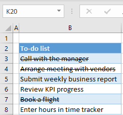
You may want to format some cells with strikethrough in Excel. Say you have the to-do list below and want to emphasize that some items are removed from the list, have been completed, or are no longer available.
As you can see, there are six items on the to-do list above. Say you have completed the tasks in B3, B4, and B7 and want to format them with strikethrough.
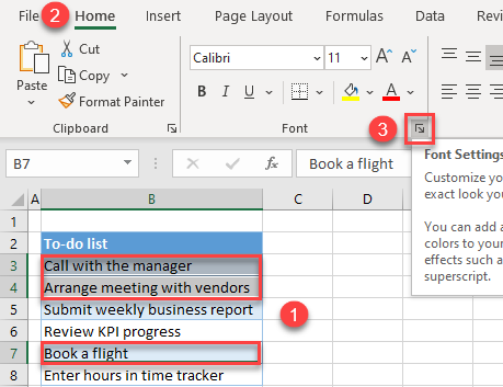
- Select cells B3, B4, and B7. Note that you can apply strikethrough to either a single cell or multiple cells at once.
- Then in the Ribbon, go to the Home tab, and in the Font section, click the Font Settings icon.
OR use the keyboard shortcut CTRL + 1.
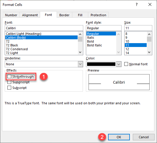
- In the Font Settings window, check Strikethrough and click OK.

Now cells B3, B4, and B7 appear to be crossed out.
Remove Strikethrough
To remove the strikethrough effect from cells, follow the steps above, but uncheck Strikethrough in Step 3 instead of checking it.
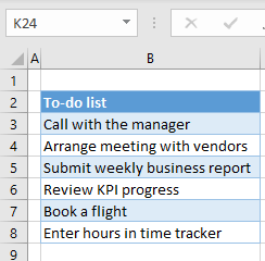
As a result, the strikethrough effect in cells B3, B4, and B7 is removed.
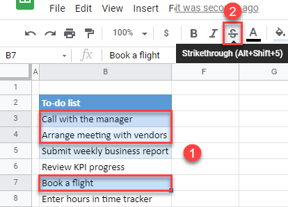
Add Strikethrough in Google Sheets
To add strikethrough in Google Sheets, select cells B3, B4, and B7 and click the Strikethrough icon in the Toolbar.
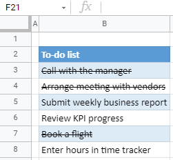
Now, the selected cells have strikethrough formatting applied.
To remove strikethrough, follow the same steps.
Also see
