How to Make Subscripts and Superscripts in Excel
Written by
Reviewed by
Last updated on July 18, 2023
This tutorial demonstrates how to make subscripts and superscripts with text formatting in Excel.
Make a Cell Subscript
To make the text in a cell subscript, follow these steps:
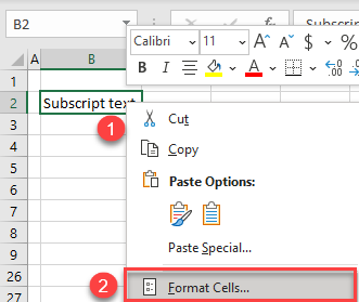
- Select the cell (e.g., B2) and right-click it, then choose Format Cells.
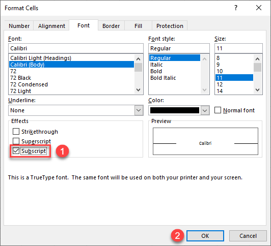
- In the Format Cells window, check Subscript and click OK.
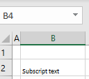
As a result, all text in cell B2 is now formatted as a subscript.
To apply the subscript or superscript format to just some of the characters in a cell, keep reading.
Make a Character Superscript
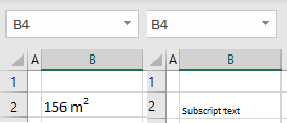
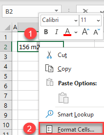
You can also make a part of the text subscript or superscript. Say you have “156 m2” in B2 and want to display the 2 as superscript (so “m2” reads as “square meters”).
- Select just the number 2 in cell B2 and right-click. Choose Format Cells.
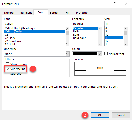
- In the Format Cells window, check Superscript and click OK.
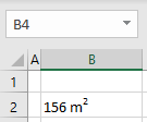
Finally, the 2 is now superscript, and the square meter unit is appropriately displayed.
See also
