How to Fix Pivot Table Field Name Not Valid Error in Excel and Google Sheets

This tutorial demonstrates how to fix a pivot table field name that is not valid in Excel and Google Sheets.

 

 

Invalid Pivot Table Field Name

To create a pivot table in Excel, the data in your worksheet must be setup in a certain format. Excel does not like blank column names, or blank columns within its data! This tutorial troubleshoots some of the reasons for this error occurring.

Missing Column Names

To create a pivot table, you need a row of column headers in the first row of your data. If any of the columns in the first row of your data is blank, you get an error message.

 

 

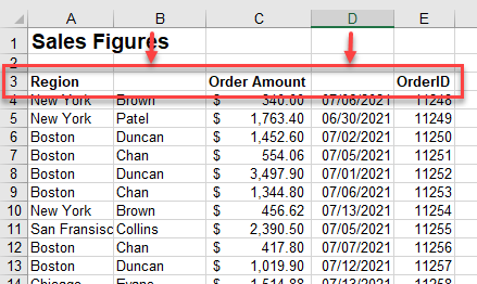
1. Make sure you have column names in each cell of the first row.

 

 

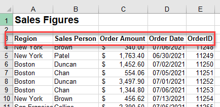
2. Then try to create the pivot table again.

Blank Columns

Hidden blank columns can also cause the field name error.

 

 

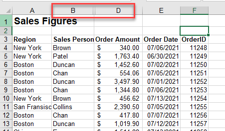
Select the columns on either side of the hidden column or columns, right-click with the mouse, and then click Unhide to show the hidden columns.

 

 

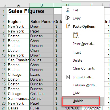
Once the column is visible, right-click the column(s) and click Delete to remove the column.

 

 

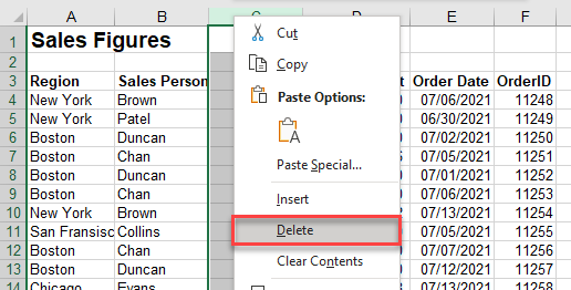
You can then try to insert your pivot table once again.

Merged Cells

If you have a heading with merged cells, you can get the field name error.

 

 

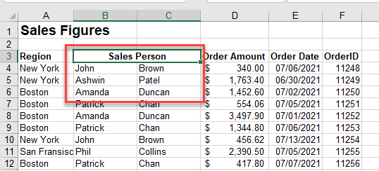
In the above example, although the Sales Person heading has been merged across Columns B and C, the actual names are separated into two columns.

To fix this, either:
Unmerge B3 and type in First Name and Surname;
OR
Concatenate the names together into one column and remove the merged header.

 

 

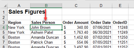
Then you can successfully insert a pivot table using the data.

Pivot Table Field Name Error in Google Sheets

Google Sheets is not as fussy as Excel when there are blank column names or hidden columns in a sheet. It creates the pivot table anyway. Then it is up to you as the user to make sure that the rows, columns, and values you insert into the pivot table return the correct data.

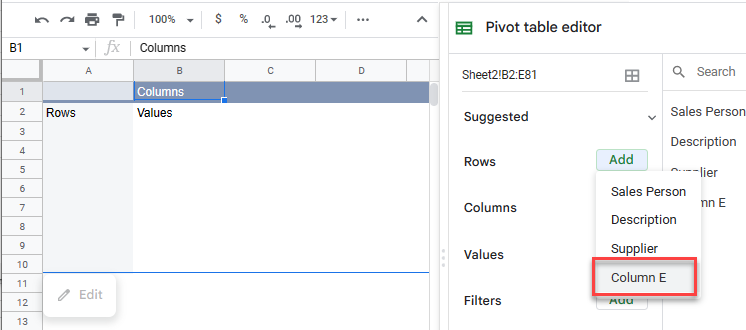
1. In the following example, the data is laid out in a format that is compatible with creating a pivot table. However, there is no heading in cell E2.

 

 

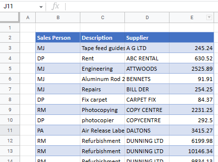
2. When you create a pivot table with this data, Google Sheets just sets a field name (here, Column E) for the unnamed column; the other fields show up with their Row 2 headings.

 

 

3. You can use the data in your pivot from the unnamed column as you would with a named column.

 

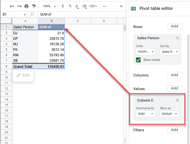
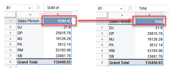
4. The only “error” that occurs is that the column name is missing; the field shows only SUM of. To solve this problem, type your own name into the pivot field’s value header.

 

Tip: Try using some shortcuts when you’re working with pivot tables.