How to Group Pivot Tables by Date in Excel
Written by
Reviewed by
This tutorial demonstrates how to group dates in Excel pivot tables.
When you add a date field (from a column of dates in the source data) to a pivot table, Excel groups the dates automatically.
Read on to see how automatic date grouping works, how to change which group fields are included, and some other grouping options. Then, see how to turn off automatic date grouping and group manually. Finally, see a common grouping error and how to fix it.
Tip: Try using some shortcuts when you’re working with pivot tables.
Group Pivot Table by Date
Consider the data table below.
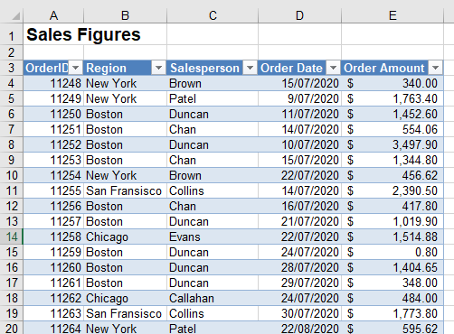
This sales data has five individual columns and is made up of 800 rows of orders. For this example Region is added to the filter area, Order Date to the row area, and Order Amount to the value area of the pivot table.
Drill Down in Automatic Date Groups
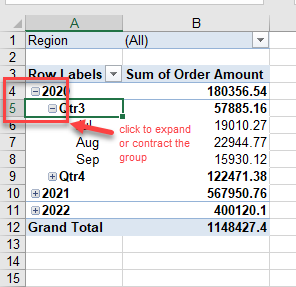
When you add a date to the filter, row, or column areas of a pivot table, Excel groups the data automatically into years and quarters. Each group has an expand (+) icon attached to it. If you click this icon, it changes to a collapse (–) icon.
Dates as Pivot Table Fields
The row area of the pivot fields reflects that, as well as the Order Date, Quarters and Years fields are created and added to the pivot table.
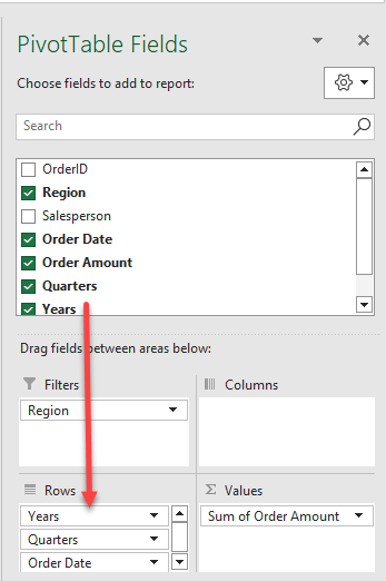
The date field itself is therefore grouped by year, quarter, and month. You can remove any of these fields, but if you remove the year, for example, then the data isn’t divided into individual years, so here, all the orders for February are included in Quarter1 > February, regardless of what year the order is in.
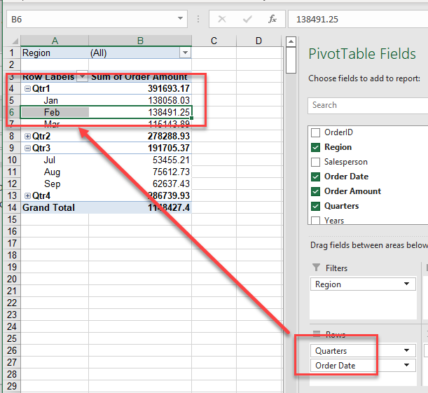
Similarly, if you remove the Quarters field, the pivot table only shows months – so all the orders in February, regardless of the year, are shown in February.
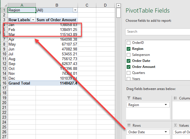
This is because, by default, pivot tables don’t group by individual dates.
Change Grouping Options
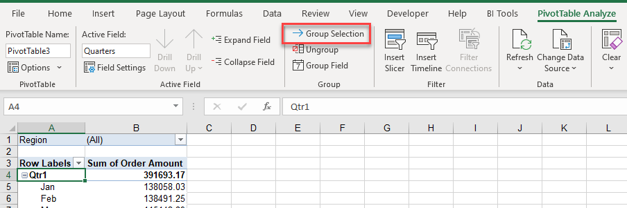
- To change the way that the pivot table groups, select the row field in the pivot table and then, in the Ribbon, go to Pivot Table Analyze > Group > Group Selection.
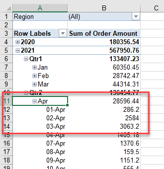
- You can now add the actual date of the order (Days) to the pivot table as well.
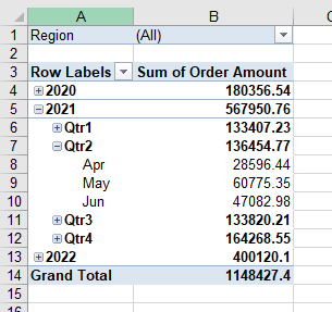
- This enables you to drill down further and expand by year, then by quarter, then by month to obtain the sales order amount for each individual day.
- Similarly, you can remove the months grouping and group just by quarters and years.
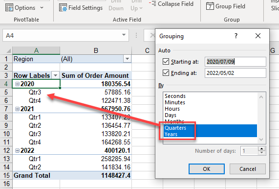
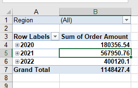
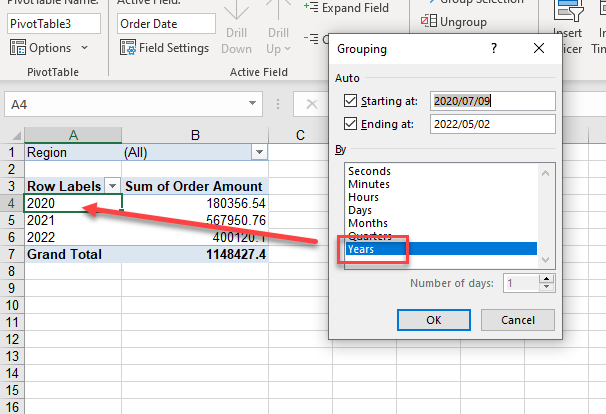
- Or, remove both the months and quarters grouping and group just by year. This gives you the order amounts for each year and removes the ability to drill down to the individual quarters, months, or dates.
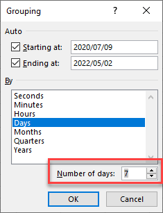
Group Pivot Data by Week
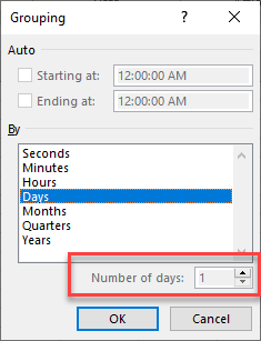
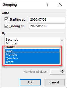
If you want to group by week, click Days in Grouping By and change the Number of days to 7. For the number of days spin button to be available, first remove grouping by Months, Quarters, and Years; do this by clicking each on them individually.
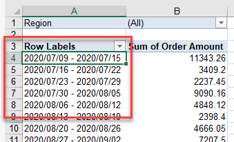
Your pivot table now displays the date field in weekly groups.
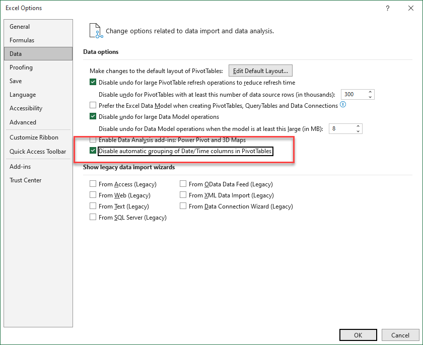
Turn Off Automatic Date Grouping
If you want Excel to keep date formatting, you can switch off automatic date grouping in a pivot table.
- In the Ribbon, go to File > Options > Data.
- Tick Disable automatic grouping of Date/Time columns in PivotTables, and then click OK.
Manual Pivot Table Grouping
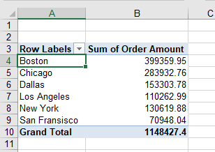
Excel allows for grouping data as you wish once the automatic date grouping is turned off. Here’s an example of manual grouping.
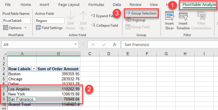
- Click in the Ribbon, and then go to PivotTable Analyze.
- Hold down the SHIFT key and click the field values to group on.
- In the Ribbon, go to PivotTable Analyze > Group > Group Selection.
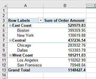
The values you chose are grouped together.
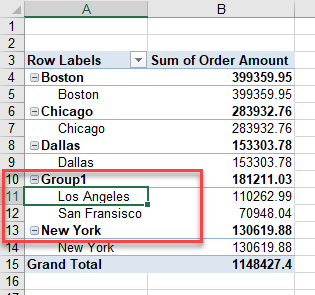
- Click in the group name (e.g., Group 1) and type in a relevant name for your group.
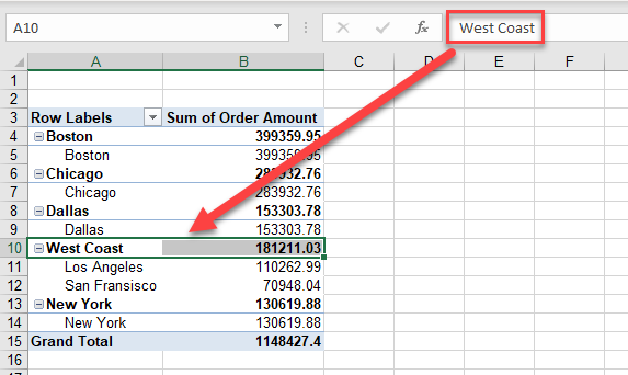
- You can then choose other values to group on (e.g., Boston and New York). Remember to hold down the SHIFT key to select multiple values. Once you have your values grouped together, you can rename those groups too.
There are no dates in the example above, but the same idea applies when grouping dates manually. You can, for example, group by four-quarter accounting period that starts at the last quarter of the prior year instead of the calendar year; it may be best to group data like that manually. Or, keep year grouping on all years starting in 2020 but group all prior years together.
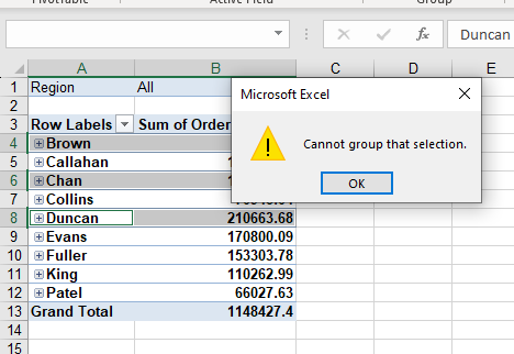
Cannot Group on That Selection
You may find that, when you are trying to group in a pivot table, you get an error saying that you cannot group that selection. If you have grouping already in place, you might not be able to add new grouping until you remove existing groups.
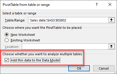
If you added the pivot table to the Data Model when you first created it, you can’t add any new levels of grouping to your data.
For example, if you have added a date field to your pivot table and then try to group by week, you cannot. The Number of days setting is disabled.