Show or Hide AutoFilter Arrows in Excel & Google Sheets
Written by
Reviewed by
This tutorial demonstrates how to show or hide AutoFilter arrows in Excel and Google Sheets.
Show AutoFilter Arrows
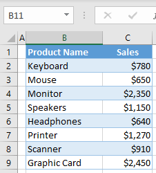
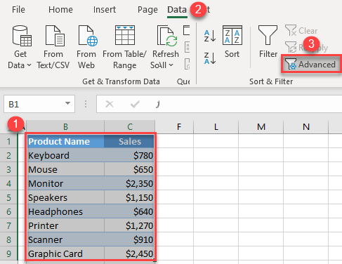
When you filter data in Excel, filter arrows appear in the heading of your data range. Say you have the following data set with Product Name in Column B and Sales in Column C.
- To display AutoFilter arrows and filter data, first click anywhere in the data range (here, B1:C9). In the Ribbon, go to Home > Sort & Filter > Filter.
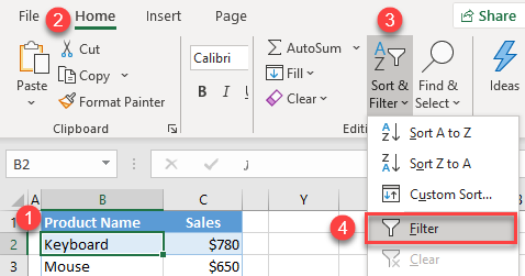
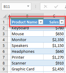
This displays AutoFilter arrows in the header data (Row 1) next to Product Name and Sales.
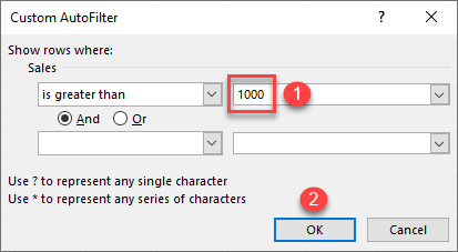
- Now say you want to filter your data, for example, to show only products that have sales greater than $1,000. Click on the filter arrow next to Sales (cell C1), go to Number Filters, and choose Greater Than…
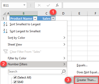
- In the pop-up window, is greater than is already set as the criteria. Type 1000 into the box to the right, and then click OK.
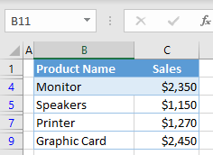
- As a result, only rows with Sales in Column C greater than $1,000 are displayed (with the row numbers highlighted in blue).
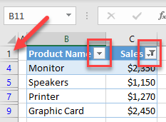
As you can see, AutoFilter arrows in the header row are still displayed. Read on for how to hide these arrows.
Hide AutoFilter Arrows
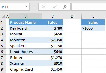
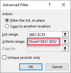
To filter data while hiding AutoFilter arrows, use an advanced filter. Let’s use the same example with Product Name and Sales. Add criteria value(s) in form of a table with the same heading name (Sales) and criteria value (>1000) somewhere out of the filtering range. In this example, the criteria range is E1:E2.
Now you can filter while hiding AutoFilter arrows.
- Select the range you want to filter (here, B1:C9) and in the Ribbon, go to Data > Sort & Filter > Advanced.
- In the Advanced Filter window, select the Criteria range (here, E1:E2), and press OK.
The result looks just like it did with standard filtering (see Step 4 image in the section above). The only difference is the “hidden” arrows in Row 1.
Show AutoFilter Arrows in Google Sheets
- To add AutoFilter arrows in Google Sheets, first click anywhere in the dataset.
- Then click the Create a filter icon in the Toolbar.
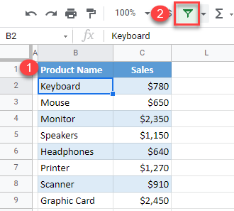
This adds AutoFilter arrows to the header row, so you can filter your data.
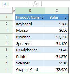
In Google Sheets, you can’t hide AutoFilter arrows while you filter data. The only way to get rid of the arrows is to remove the filter.
