How to Show Only Duplicates in Excel & Google Sheets

This tutorial demonstrates how to show only duplicates in Excel and Google Sheets.

 

 

Show Only Duplicates

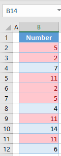
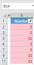
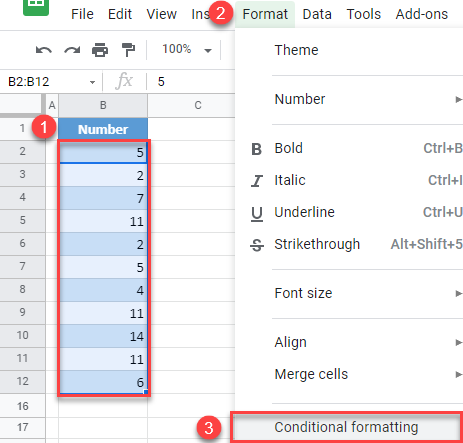
Say you have the list of numbers pictured below and want to display only duplicate values.

 

 

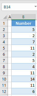
The numbers 5, 2, and 11 are listed twice in Column B. To display only those values, you can use conditional formatting to highlight the cells with duplicate values, then filter by color to extract them.

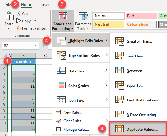
1. First, create a conditional formatting rule for duplicate values in the list.
   Select the range with duplicates (here, B2:B12) and in the Ribbon, go to Home > Conditional Formatting > Highlight Cells Rules > Duplicate Values.

 

 

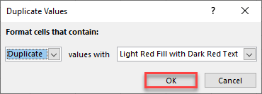
2. In the pop-up window, leave the default options (Duplicate and Light Red Fill with Dark Red Text) and click OK.

 

 

As a result, all cells with duplicate values are highlighted in red.

 

 

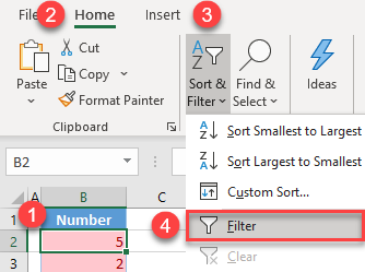
3. Next, turn on filtering. Click on any cell in the data range (B1:B12), and in the Ribbon, go to Home > Sort & Filter > Filter.

 

 

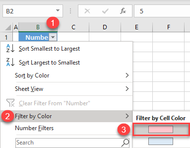
4. Click on the filter button next to Number (cell B1), go to Filter by Color, and choose red.

 

 

As a result of this step, only cells with duplicate values are displayed.

 

 

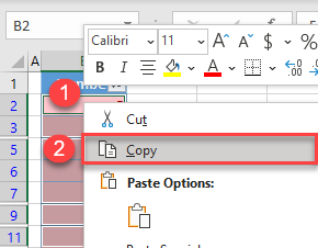
5. Now copy only the filtered values to Column C.
   Select all filtered cells and right-click in the selected area, and click Copy (or use the keyboard shortcut CTRL + C).

 

 

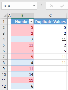
6. Right-click cell C2 and choose Values under Paste Options.

 

 

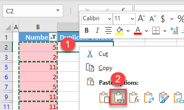
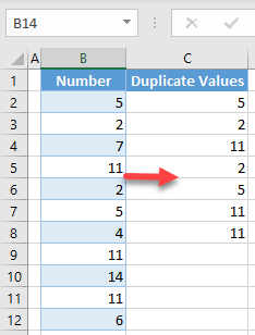
Finally, all duplicate values from Column B, are copied into Column C.

 

 

Show Only Duplicates in Google Sheets

Let’s use the same example to explain how to show only duplicates in Google Sheets.

1. Select the data range with numbers (B2:B12) and in the Menu, go to Format > Conditional formatting.

 

 

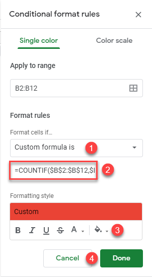
2. In the Conditional Formatting window, (1) for Format rules choose Custom formula is, then (2) enter the formula:

=COUNTIF($B$2:$B$12,$B2) > 1

This formula checks, for each cell, how many times that value appears in the range B2:B12. If it appears more than once, that means there are duplicate values for the cell, and it should be highlighted in red.
Then (3) set red as the fill color and (4) click Done.

 

 

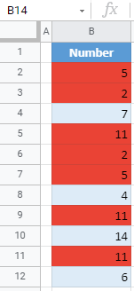
When this conditional formatting rule is applied, all duplicate values have a red background color.

 

 

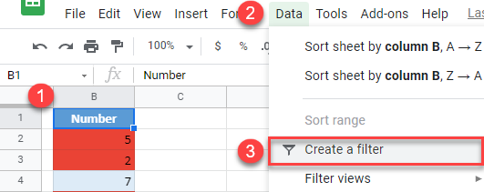
3. Now to turn on filtering, click on cell B1 and in the Menu go to Data > Create a filter.

 

 

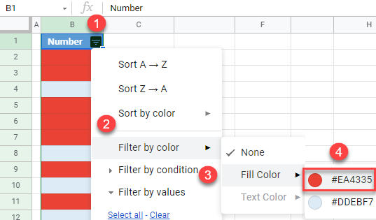
4. Click on the (1) filter button next to Number (cell B1), (2) go to Filter by color, (3) click Fill Color, and (4) choose red (#EA4335).

 

 

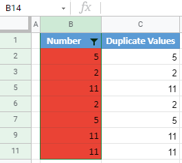
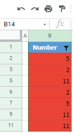
Now only duplicate values, highlighted in red, are displayed. All other cells are hidden.

 

 

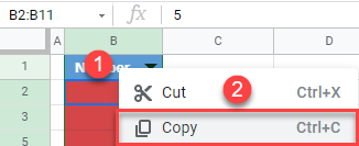
5. To copy the filtered cells, select them and right-click anywhere in the selected range, then click Copy (or use the keyboard shortcut CTRL + C).

 

 

6. Right-click in cell C2, select Paste special, and choose Paste values only (or use the keyboard shortcut, CTRL + SHIFT + V).

 

 

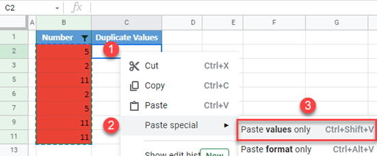
As a result, only duplicate values are copied into Column C.