Cumulative/ Moving (Rolling) Average – Excel and Google Sheets
This tutorial will demonstrate how to calculate a rolling average in Excel and Google Sheets.
Moving Average is used in time series data analysis to smoothen out short-term fluctuations in a dataset and thus be able to highlight and predict longer-term trends or cycles. The moving average can be calculated as a simple, weighted, or exponential moving average.
The Simple Moving Average calculates the moving average of a subset of data points where all data points have the same weight. That is, all data points are treated equally. In this article, we will look at how to calculate the cumulative average and the simple moving average.
Cumulative Average Formula
The cumulative average (CA) is calculated using the formula:
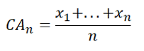
where x1+…+xn are the data values from the first value to the current value;
CAn is the cumulative average of the current data point;
n is the count from the first data point to the current data point.
Simple Moving Average Formula
The k-data points Simple Moving Average (SMAk) is calculated using the formula:
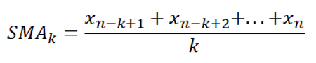
where xn-k+1 + xn-k+2 + … + xn are the current data value and the previous k-1 data values;
SMAk is the simple moving average of k data points up to the current data point; and
k is the desired fixed subset of the dataset.
Calculate Cumulative Average and Simple Moving Average in Excel
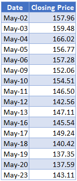
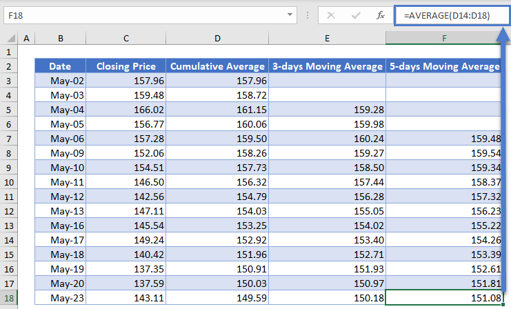
Background: The closing prices of Apple Inc. stock on NASDAQ for the sixteen trading days from 2nd to 23rd May 2022 are shown in the table below. Calculate the cumulative averages of the stock prices over the 16 trading days as well as the 3-days, and the 5-days moving averages for the stock prices.
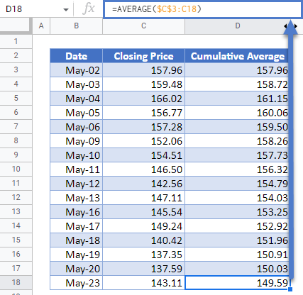
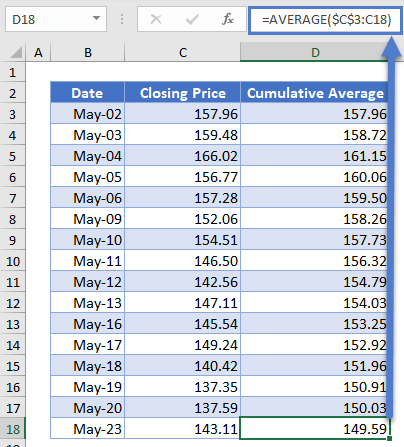
First, calculate the cumulative averages of the stock prices using the AVERAGE Function.
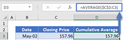
Notice that we used absolute referencing (the dollar sign) for the first value of the average function and did not use it for the second value. This is because, when calculating the cumulative average, we must start from the beginning of the dataset to the current value. You will notice that when you autofill the rest of the column, the second value changes to the cell of the current value.
Note: Double-Click the bottom right corner of the cell to fill down the data to the rest of the column.
The complete Cumulative Average column is shown below.
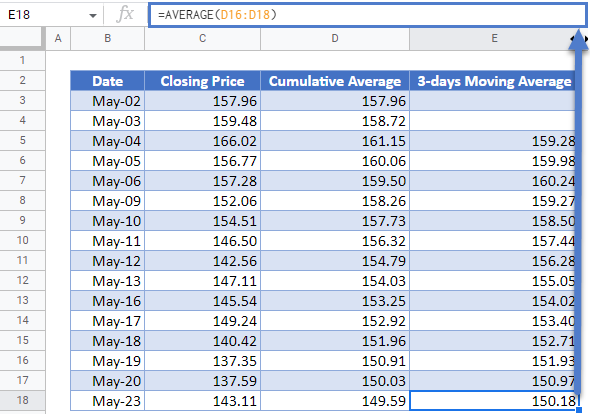
Next, calculate the 3-days moving average. We will start from the 3rd data, i.e. May-04, and use the AVERAGE Function to calculate the average of the stock prices of the current data point and the previous data points. That is, the 3-days Moving Average for the stock prices on May-04 is the average of the stock prices of May-04, May-03, and May-02. The 3-days Moving Average for the stock prices on May-05 is the average of the stock prices of May-05, May-04, and May-03, and so on. The calculation is shown below.
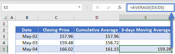
Note that we did not use the dollar sign in any of the cells in the AVERAGE Function because we want the cells to recalculate accordingly when we autofill the rest of the column.
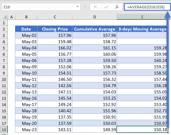
Autofill the rest of the column and you have the complete 3-days Moving Average column as shown below.
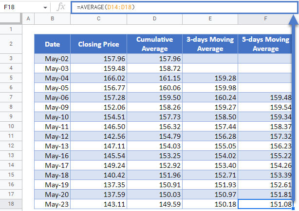
Next, calculate the 5-days moving average in a similar way as the 3-days moving averages except that this time you start from the fifth data and use 5 days as the range for the AVERAGE Function.
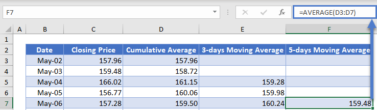
Autofill the rest of the column and you have the complete 5-days Moving Average column as shown below.
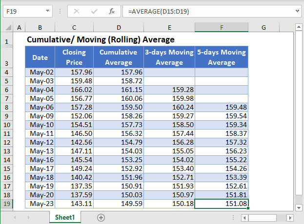
Cumulative Averages and Moving Averages in Google Sheets
Cumulative Averages and Moving Averages can be calculated in Google Sheets in a similar way as it is calculated in Excel as shown in the pictures below.