Highlight Duplicate Values – Excel & Google Sheets

This tutorial will demonstrate how to highlight cells in a range of  cells where there are duplicate values using Conditional Formatting in Excel and Google Sheets.

 

 

Conditional Formatting – Highlight Duplicate Values

Duplicate Cell Rule

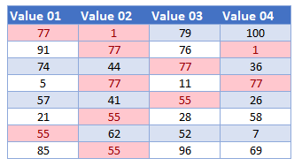
To highlight cells with duplicate values, use the built-in duplicate value rule within the Conditional Formatting menu option. (You can also highlight the whole row.)

1. Select the range you want to apply formatting to.
2. In the Ribbon, select Home > Conditional Formatting > Duplicate Values.

 

 

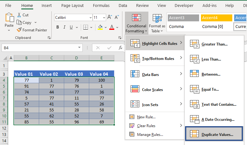
3. Select the format you require.

 

 

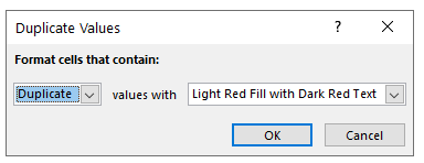
4. Click OK to see the result.

 

 

Create a New Rule

You can highlight cells where there are duplicate values in a range of cells by creating a New Rule in Conditional Formatting.

1. Select the range you want to apply formatting to.
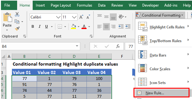
2. In the Ribbon, select Home > Conditional Formatting > New Rule.

 

 

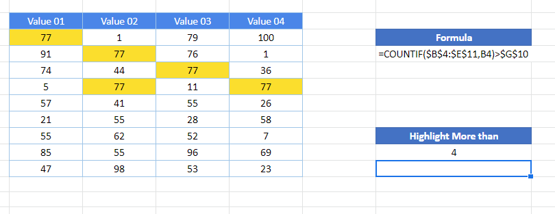
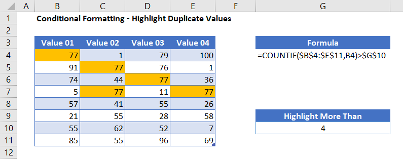
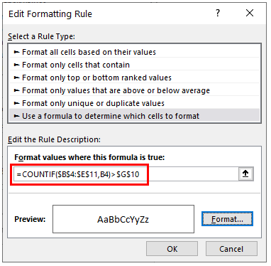
3. Select Use a formula to determine which cells to format, and enter the COUNTIF formula:

=COUNTIF($B$4:$E$11,B4)>$G$10

 

 

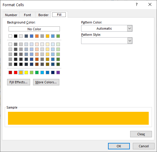
4. Click on the Format button and select your desired formatting.

 

 

5. Click OK, and then OK once again to return to the Conditional Formatting Rules Manager.

 

 

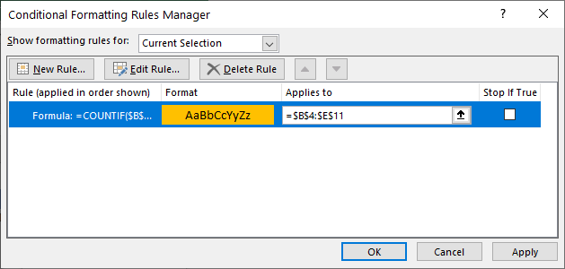
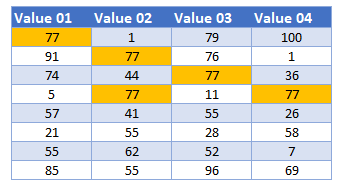
6. Click Apply to apply the formatting to your selected range and then click Close. The result will show you how many numbers appear more than four times in your range.

 

 

Highlight Duplicate Values in Google Sheets

Use a custom function to highlight duplicate values in Google Sheets.

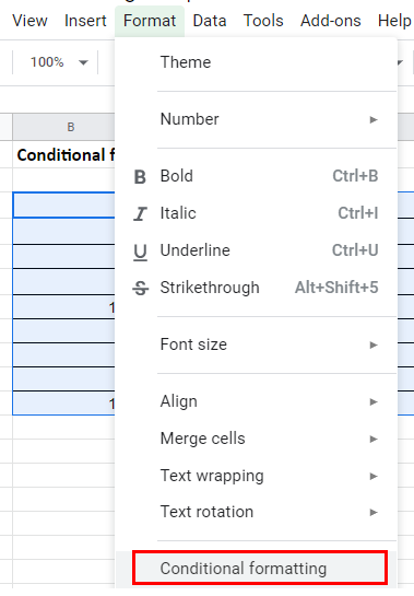
1. Highlight the cells you wish to format, and then click on Format > Conditional Formatting.

 

 

2. The Apply to Range section will already be filled in.

 

 

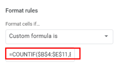
3. From the Format Rules section, select Custom Formula from the drop-down list and type in the following formula to look for text at the beginning of your cell.

=COUNTIF($B$4:$E$11,B4)>$G$10

 

 

4. Select the fill style for the cells that meet the criteria.

 

 

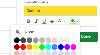
5. Click Done to apply the rule. In this case we are highlighting cells with duplicate values, that is, with two or more repetitions.

 

 

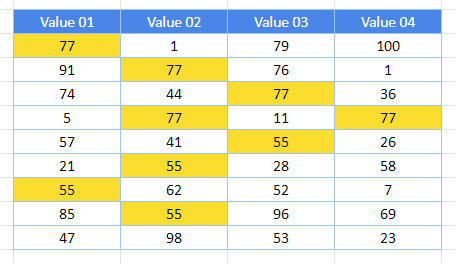
6. Change the value in G10 to see the results change accordingly.