Find Last Row with Data – Excel & Google Sheets

This tutorial will demonstrate how to find the last non-blank row in a dataset in Excel and Google Sheets.

Find the Last Row with Data

It’s often useful to know at which row your data ends. If your range has or can have blank cells, you can find the last non-blank row using one of the methods below.

Universal Method

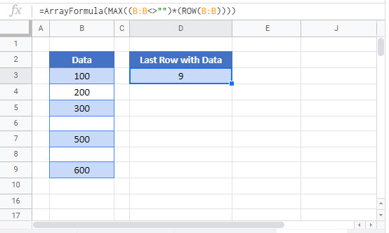
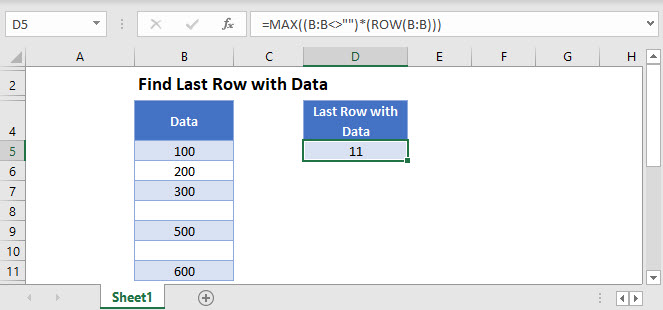
The first method uses the ROW and MAX Functions and can be used with any kind of data:

=MAX((B:B<>"")*(ROW(B:B)))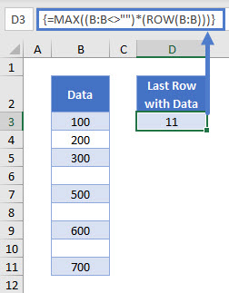

Let’s analyze this formula.

We start by using a logical test on the data column. Our formula looks at the entire column (B:B) and outputs TRUE for non-blank cells and FALSE for blank cells.

=B:B<>""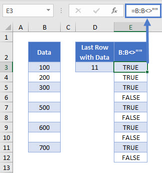

The ROW Function produces the row number of a given cell. If we don’t give it a specific cell input, it gives the row number of the cell it’s in.

=ROW()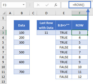

Multiplying each row number by the corresponding TRUE (= 1) or FALSE (= 0) values, returns the row number for a populated cell, and zero for a blank cell.

=E3*F3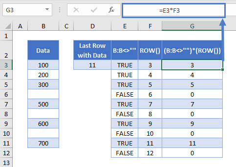

The MAX Function gives the maximum of a set of numbers. In this example, since all blank cells produce a zero value, the maximum is the highest row number.

=MAX(G3:G12)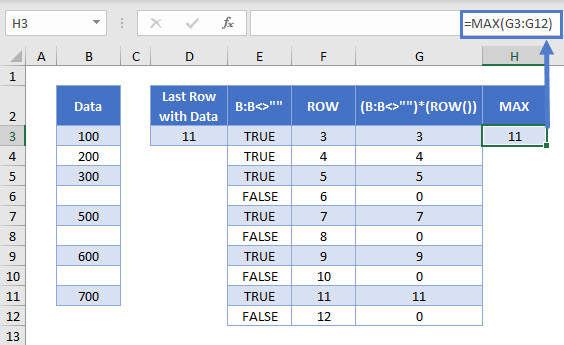

Combining these steps gives us our original formula:

=MAX((B:B<>"")*(ROW(B:B)))

Please note that this is an array formula, so if you’re using Excel 2019 or earlier, you have to press CTRL + SHIFT + ENTER to trigger it.

Method for Text Range

If your (non-continuous) range contains only text values and blank cells, you can use a less complicated formula containing the REPT and MATCH Functions:

=MATCH(REPT("z",50),B:B)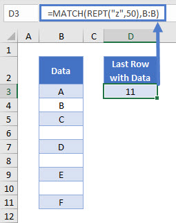

Let’s see how this formula works.

REPT Function

The REPT Function repeats a text string a given number of times. For this example, we can use it to create a text string which would be the last in any alphabetically sorted list. If we repeat “z” 50 times, this should work for almost any text data column; no entries would come before “zzzzzzzzzzzzzzzzzzzzzzzzzzzzzzzzzzzzzzzzzzzzzzzzzz” alphabetically.

=REPT("z",50)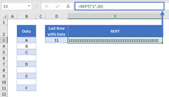

MATCH Function

The MATCH Function finds a given lookup value in an array.

We perform a search of the entire data column for our 50-z text string. Omitting the match type input in the MATCH Function tells it to find an approximate rather than an exact match.

=MATCH(REPT("z",50),B:B)

The MATCH Function searches through Column B and looks for our text string of 50 “z”s. Since it does not find it, the formula returns the position of the last non-blank cell. This cell contains the last value in the lookup array that’s less than (or equal to) the lookup value.

Keep in mind that this formula works only when your range contains exclusively text and blank cells (or at least the last cell’s value is non-numeric).

Find Last Row With Data in Google Sheets

These formulas work exactly the same in Google Sheets as in Excel.