Find Missing Values – Excel & Google Sheets

This tutorial will demonstrate how to check whether items are missing within a list in Excel and Google Sheets.

Find Missing Values

There are several ways to check if items are missing from a list.

Find Missing Values with COUNTIF

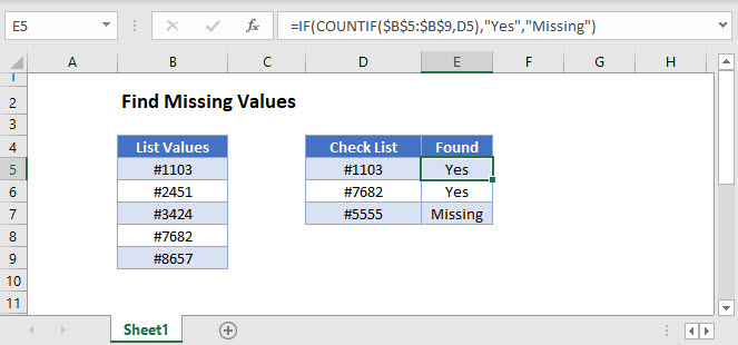
One way to find missing values in a list is to use the COUNTIF Function together with the IF Function.

=IF(COUNTIF(B3:B7,D3),"Yes","Missing")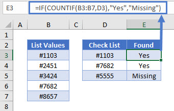

Let’s see how this formula works.

COUNTIF Function

The COUNTIF Function counts the number of cells that meet a given criterion. If no cells meet the condition, it returns zero.

=COUNTIF(B3:B7,D3)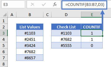

In this example, “#1103” and “#7682” are in Column B, so the formula gives us 1 for each. “#5555” is not in the list, so the formula gives us 0.

IF Function

The IF Function will evaluate any non-zero number as TRUE, and zero as FALSE.

Within the IF Function, we perform our count, then output “Yes” for TRUE and “No” for FALSE. This gives us our original formula of:

=IF(COUNTIF(B3:B7,D3),"Yes","Missing")

Find Missing Values with VLOOKUP

Another way to find missing values in a list is to use the VLOOKUP and ISNA Functions together with the IF Function.

=IF(ISNA(VLOOKUP(D3,B3:B7,1,FALSE)),"Missing","Yes")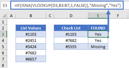

Let’s go through this formula.

VLOOKUP Function

Start by performing an exact-match VLOOKUP (FALSE) for the values in your list.

=VLOOKUP(D3,B3:B7,1,FALSE)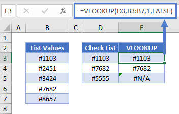

If the item is found, the VLOOKUP Function will return that item, otherwise it will return the #N/A error.

ISNA Function

You can use the ISNA Function to convert the #N/A errors to TRUE, indicating that those values are missing.

=ISNA(E3)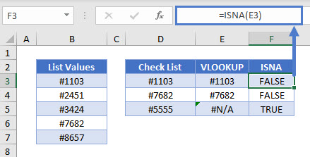

All non-error values result in FALSE.

IF Function

Then convert the results of the ISNA Function to show whether the value is missing. If the VLOOKUP Function gave us an error, the item is “Missing”.

=IF(F3,"Missing","Yes")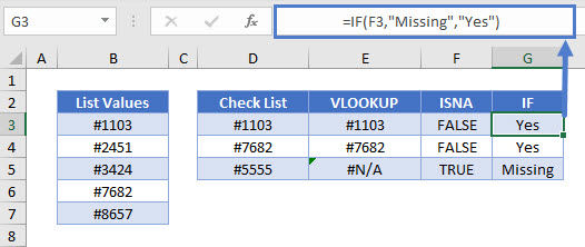

Item in both lists display “Yes”.

Combining these steps gives us the original formula:

=IF(ISNA(VLOOKUP(D3,B3:B7,1,FALSE)),"Missing","Yes")

Find Missing Values in Google Sheets

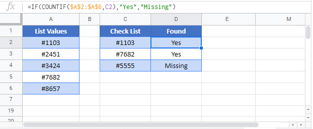
These formulas work exactly the same in Google Sheets as in Excel.