Remove Numbers From Text in Excel & Google Sheets

This tutorial will demonstrate how to remove numbers from text in a cell in Excel & Google Sheets.

We will discuss two different formulas for removing numbers from text in Excel.

SUBSTITUTE Function Formula

We can use a formula based on the SUBSTITUTE Function. It’s a long formula but it’s one of the easiest ways to remove numbers from an alphanumeric string.

In this formula, we have nested SUBSTITUTE functions 10 times (one for each number: 0,1,…,9), like this:

=SUBSTITUTE(SUBSTITUTE(SUBSTITUTE(SUBSTITUTE(SUBSTITUTE(SUBSTITUTE(SUBSTITUTE(SUBSTITUTE(SUBSTITUTE(SUBSTITUTE(
B3,1,""),2,""),3,""),4,""),5,""),6,""),7,""),8,""),9,""),0,"")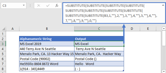

Array TEXTJOIN formula

To remove numbers from alphanumeric strings, we can also use a complex array formula that consists of the TEXTJOIN, MID, ROW, and INDIRECT functions.

{=TEXTJOIN("",TRUE,IF(ISERR(MID(B3,ROW(INDIRECT("1:"&LEN(B3))),1)+0),MID(B3,ROW(INDIRECT("1:"&LEN(B3))),1),""))}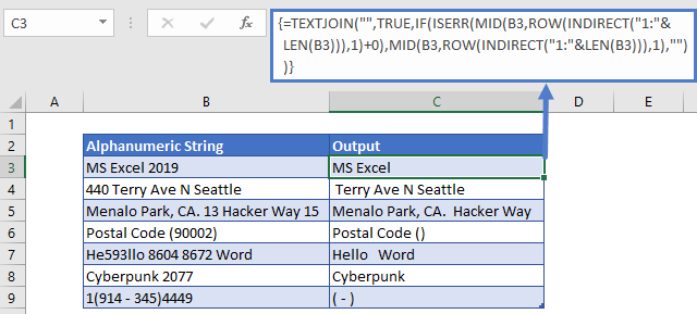

Note: TEXTJOIN is a new Excel Function available in Excel 2019+ and Office 365.

This is a complex formula, so we’ll divide it into steps to understand it better.

Step 1

The MID Function is a Text Function that returns text from the middle of a cell. You must indicate the number of characters to return and the start character.

For the start number (start_num) argument in the MID function, we’ll use the resultant array list from the ROW and INDIRECT functions.

=ROW(INDIRECT("1:"&LEN(B3)))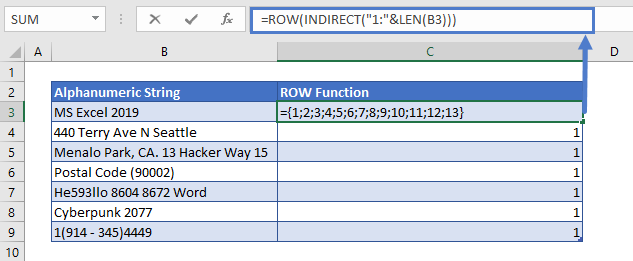

For the number of characters (num-chars), use 1. After entering the arguments in the MID function, it will return an array.

{=MID(B3,ROW(INDIRECT("1:"&LEN(B3))),1)}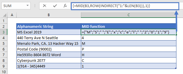

Step 2

We’ll add zero (+ 0) to each value in the resultant array (that we get from the above MID function). In Excel, if numbers are added to non-numeric characters, we’ll get a #VALUE! Error. So, after adding 0 in the above array, we’ll get an array of numbers and #Value! Errors.

{=MID(B3,ROW(INDIRECT("1:"&LEN(B3))),1)+0}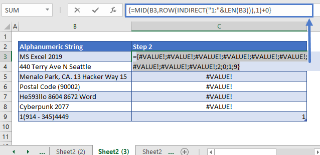

Step3

Next use the ISERR Function to return TRUE for errors and FALSE for non-error values, outputting an array of TRUE and FALSE, TRUE for non-numeric characters, and FALSE for numbers.

=ISERR(MID(B3,ROW(INDIRECT("1:"&LEN(B3))),1)+0)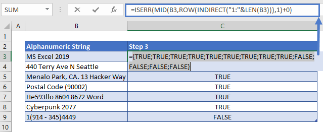

Step 4

Next add the IF Function.

The IF function will check the result of the ISERR function (Step 3). If its value is TRUE, it will return an array of all the characters of an alphanumeric string. For this, we have added another MID function without adding zero at the end. If the value of the IF function is FALSE, it will return blank (“”).

In this way, we’ll have an array that contains only the non-numeric characters of the string.

=IF(ISERR(MID(B3,ROW(INDIRECT("1:"&LEN(B3))),1)+0),MID(B3,ROW(INDIRECT("1:"&LEN(B3))),1),"")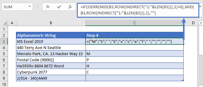

Step 5

Finally, the above array is put into the TEXTJOIN function. The TEXTJOIN function will join all the characters of the above array and ignore the empty string.

The delimiter for this function is set an empty string (“”) and the ignore_empty argument’s value is entered TRUE.

This will give us the desired result i.e. only the non-numeric characters of the alphanumeric string.

{=TEXTJOIN("",TRUE,IF(ISERR(MID(B3,ROW(INDIRECT("1:"&LEN(B3))),1)+0),MID(B3,ROW(INDIRECT("1:"&LEN(B3))),1),""))}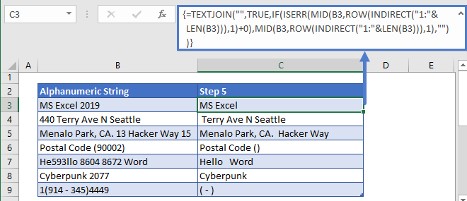

Note: This is an Array Formula. When entering array formulas in Excel 2019 or earlier, you must use CTRL + SHIFT + ENTER to enter the formula instead of the regular ENTER.

You’ll know you entered the formula correctly by the curly brackets that appear. DO NOT manually type the curly brackets, the formula will not work.

With Office 365 (and presumably versions of Excel after 2019), you can simply enter the formula like normal.

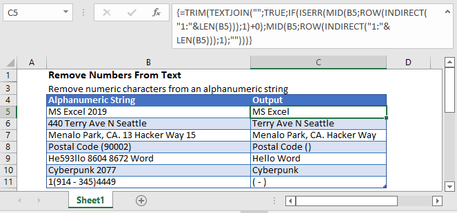
TRIM Function

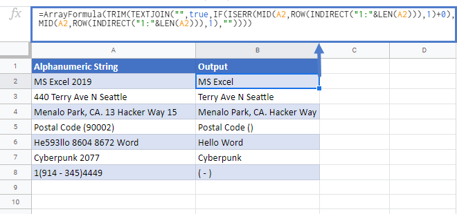
When the numbers are removed from the string, we might have extra spaces left. To remove all the trailing and leading spaces, and the extra spaces between words, we can use the TRIM function before the main formula, like this:

=TRIM(C3)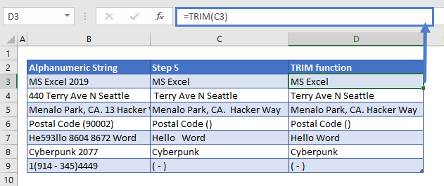

Remove Numbers from Text In Google Sheets

The formula to remove numbers from the text works exactly the same in Google Sheets as in Excel: