Reverse the Order of a List / Range – Excel & Google Sheets
Written by
Reviewed by
Download the example workbook
This tutorial will teach you how to reverse the order of a list or range in Excel & Google Sheets.
Reverse Order using INDEX Function
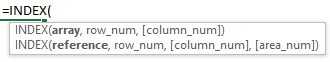
The INDEX function returns the value (can be any data type) positioned at the intersection of a specified row and column in a range or array. Its syntax is:
We can use the INDEX function to reverse the order of a list of items like this:
=INDEX(B$3:B$7,C3,1)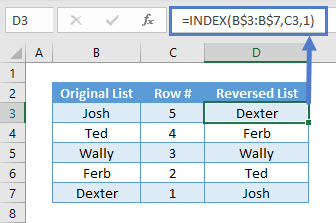
In this example, column C provides the values for the ‘row_num’ argument of the INDEX function syntax. It has been calculated using the COUNTA and the ROW function, like this:
=COUNTA(B$3:B$7)+ROW(B$3:B$7)-ROW()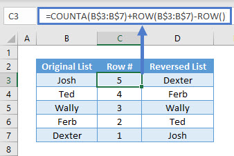
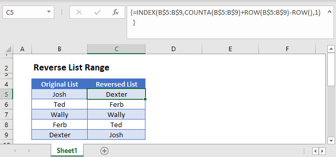
Reverse Order using INDEX, COUNTA & ROW Function
In the previous example, we split the formulas up to make it easier to follow. Instead, you can merge these formulas into one, like this:
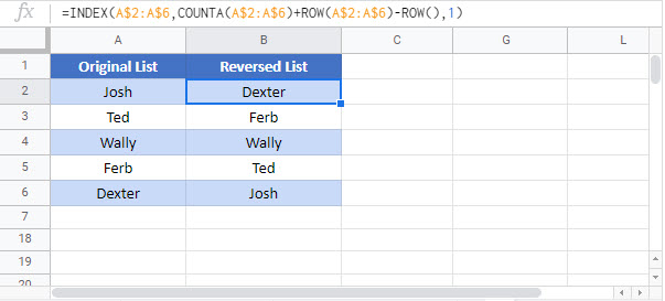
=INDEX(B$3:B$7,COUNTA(B$3:B$7)+ROW(B$3:B$7)-ROW(),1)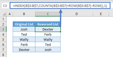
Note: Mixed cell reference has been used for the range in each of the formulas to make it easier to drag down.
Reverse the Order of a List / Range in Google Sheets
These formulas work exactly the same in Google Sheets as in Excel.