Sum By Category or Group – Excel & Google Sheets
Written by
Reviewed by
Download the example workbook
This tutorial will demonstrate how to calculate subtotals by group using the SUMIFS Function in Excel and Google Sheets.
Subtotal Table by Category or Group
This first example requires that you have access to the UNIQUE Function. This function is available in newer version of Excel, Excel 365, or Google Sheets. If you don’t have access to this function skip to the next section.
We can use the UNIQUE Function and the SUMIFS Function to automatically subtotal the Number of Products by Product Group. This is the final SUMIFS FUNCTION:
=SUMIFS(C3:C11,B3:B11,E3)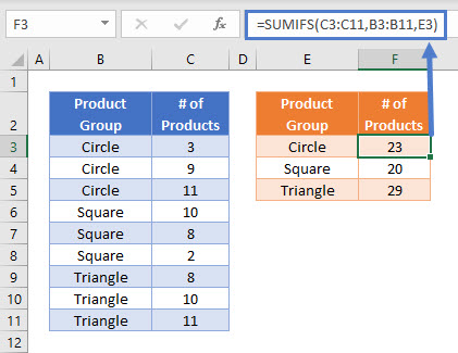
However, first, we added the UNIQUE Function to cell E3:
=UNIQUE(B3:B11)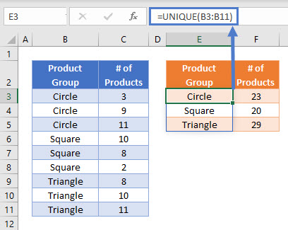
When this formula is entered, a list is automatically created below the cell to show all unique values found within Product Group.
This is a dynamic array function where the size of the results list does not need to be defined, and it will automatically shrink and grow as the input data values change.
Note that in Excel 365, the UNIQUE Function is not case sensitive, but in Google Sheets it is.
Subtotal Table by Category or Group – Without UNIQUE Function.
If you are using a version of Excel without the UNIQUE Function, you can combine the INDEX Function and MATCH Function with a COUNTIF Function to create an array formula to produce a list of unique values from a range of cells:
{=INDEX($B$3:$B$11,MATCH(0,COUNTIF($E$2:E2,$B$3:$B$11),0))}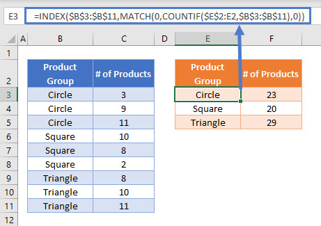
In order for this formula to function, the fixed cell references need to be written carefully, with the COUNTIF Function referencing the range $E$2:E2, which is the range starting from E2 until the cell above the cell containing the formula.
The formula also needs to be entered as an array formula by pressing CTRL + SHIFT + ENTER after it has been written. This formula is a 1-cell array formula, which can then be copy-pasted into the cells E4, E5 etc. Do not enter this as an array formula for the whole range E3:E5 in one action.
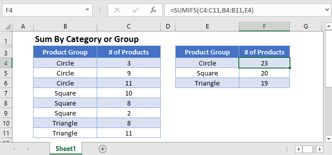
In the same way as in the previous example, a SUMIFS Function is then used to subtotal the Number of Products by Product Group:
=SUMIFS(C3:C11,B3:B11,E3)
Sum by Category or Group – Subtotals in Data Tables
Alternatively, we can add subtotals directly into a data table with the IF and SUMIFS Functions.
=IF(B3=B2,"",SUMIFS(C3:C11,B3:B11,B3))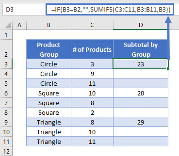
This example uses a SUMIFS Function nested within an IF Function. Let’s break down the example into steps:
We start by totaling the Number of Products that match the relevant Product Group:
=SUMIFS(C3:C11,B3:B11,B3)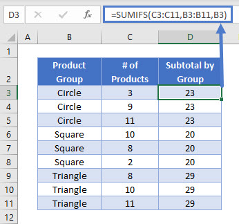
This formula produces a subtotal value for every data row. To show subtotals only in the first data row of each Product Group, we use the IF Function. Note that the data must already be sorted by Product Group to ensure that the subtotals are displayed correctly.
=IF(B3=B2,"",SUMIFS(C3:C11,B3:B11,B3))
The IF Function compares each data row’s Product Group value with the data row above it, and if they have the same value it outputs a blank cell (“”).
If the Product Group values are different, the sum is displayed. This way, each Product Group sum is displayed only once (on the row of its first instance).
Sorting Datasets by Group
If the data isn’t already sorted, we can still use the same formula for the subtotal.
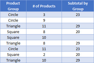
The dataset above isn’t sorted by Product Group, so the Subtotal by Group column displays each subtotal more than once. To get the data into the format we want, we can select the data table and click “Sort A to Z”.

Locking Cell References
To make our formulas easier to read, we’ve shown some of the formulas without locked cell references:
=IF(B3=B2,"",SUMIFS(C3:C11,B3:B11,B3))But these formulas will not work properly when copy and pasted elsewhere in your file. Instead, you should use locked cell references like this:
=IF(B3=B2,"",SUMIFS($C$3:$C$11,$B$3:$B$11,B3))Read our article on Locking Cell References to learn more.
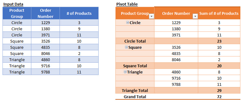
Using Pivot Tables to Show Subtotals
In order to remove the requirement to pre-sort the data by Product Group, we can use the power of Pivot Tables to summarize the data instead. Pivot Tables calculate subtotals automatically and display totals and subtotals in several different formats.
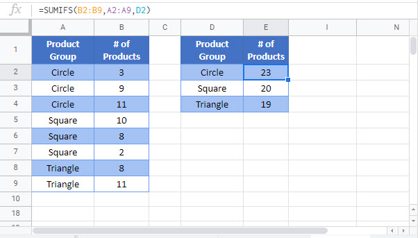
Sum by Category or Group in Google Sheets
These formulas work the same in Google Sheets as in Excel. However, the UNIQUE Function is case sensitive in Google Sheets.