Sum Text in Excel & Google Sheets

This tutorial will demonstrate how to find the sum of text values where a unique code is assigned to each such text value in Excel and Google Sheets.

SUM Numbers Stored as Text

First we will look at how to sum numbers stored or formatted as text.

In the following example, the column Salary is stored as text. If attempt to sum the values, Excel will display a zero.

=SUM(C3:C7)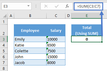

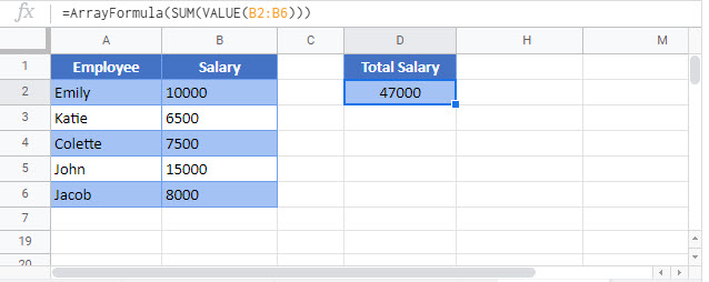
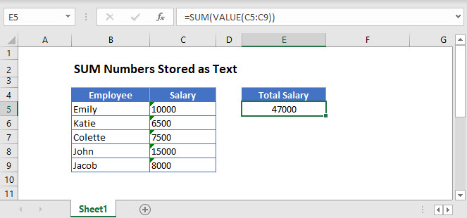
Instead, to perform the SUM Operation on numbers stored as text, you can use an array formula with the  VALUE Function like this:

=SUM(VALUE(C3:C7))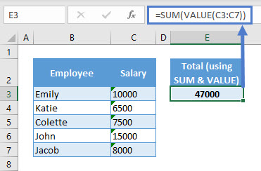

The VALUE Function converts a text representing a number to a number. The SUM Function sums those numbers.

In Excel 365 and version of Excel newer than 2019, you can simply enter the formula like normal. However, when using Excel 2019 and earlier, you must enter the array formula by pressing CTRL + SHIFT + ENTER (instead of ENTER), telling Excel that the formula is an array formula. You’ll know it’s an array formula by the curly brackets that appear around the formula (see top image). In later versions of Excel and Excel 365, you can simply press ENTER instead.

Let us look at the following explanation to get a better understanding of the formula.

VALUE Function

Used as an array formula, the VALUE Function converts the whole range of numbers stored as text to an array of numbers and returns it as an input for the SUM Function.

=SUM({10000;6500;7500;15000;8000})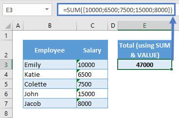

To see what the VALUE Function returns, select the required function and press F9.

SUM of Text Values

To SUM a range of text values where a unique code is assigned to each such text value, an array formula can be used.

The following table records answers for three given questions. The table on the right contains a point value for each question. We want to sum the total point values for each person.

This is the final formula:

=SUM(INDEX(I$3:I$6,N(IF(1,MATCH(C4:E4,H$3:H$6,0)))))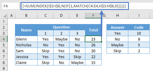

We will walk through the formula below.

MATCH Function

The MATCH Function looks for a specified item in a range and returns its relative position in that range. Its syntax is:

=SUM(INDEX(I$3:I$6,N(IF(1,{1,3,2}))))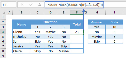

For a given person, the MATCH Function finds the relative position of each answer in the range H3:H6. The result is an array of positions.

Note: In an array formula, to view what a function returns, select the required function and press F9.

IF & N Function

The IF and the N Functions used together return the following array as an input for the INDEX Function.

=SUM(INDEX(I$3:I$6,{1,3,2}))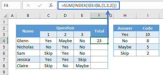

Here, the two functions return an array of relative position of answers in the range H3:H6. The purpose of using the IF and the N Functions is for performing a process called dereferencing. In simple terms, the two functions force the INDEX Function to pass on the whole array of code values to the SUM Function.

We explain this in the next section.

INDEX Function

The INDEX function returns the value positioned at the intersection of a specified row and column in a range. Its syntax is:

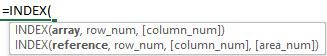
Let’s see how it works as an array formula:

=SUM({10,5,8})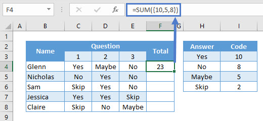

The INDEX Function finds the code values in the range I3:I6 according to the given position numbers. It then returns an array of values, i.e. the respective code for each answer, to the SUM Function to perform operations.

Make sure the number of rows and columns in both the Answer and the Code column is same.

SUM Function

The SUM Function will sum the code values returned by the INDEX Function.

=SUM({10,5,8})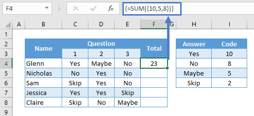

All of this put together yields our initial formula:

{=SUM(INDEX(I$3:I$6,N(IF(1,MATCH(C4:E4,H$3:H$6,0)))))}

SUM of Text Values – Without IF & N Functions

This section explains how Excel responds if we don’t use the IF and the N Function in the above mentioned formula.

The same example is being used with the same codes and answers.

{=SUM(INDEX(I$3:I$6,MATCH(C4:E4,H$3:H$6,0)))}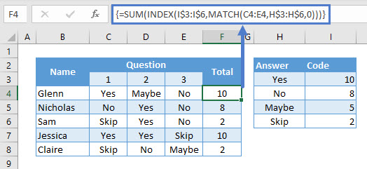

As you can see, the INDEX Function passes only the code for the first answer to the SUM Function. If you scrutinize on the INDEX Function by pressing F9 you’ll get the following:

The #VALUE! Error is returned because the INDEX Function cannot read the array of row numbers as an array. Hence, using the IF & the N Function does the trick.

Note: In Excel 365, you can skip using the IF and the N Functions altogether.

 

Sum Text– Google Sheets

These formulas work the same in Google Sheets as in Excel.