Use Cell Value in Formula – Excel & Google Sheets

This tutorial will demonstrate how to use a cell value in a formula in Excel and Google Sheets.

 

Cell Value as a Cell Reference

The INDIRECT Function is useful when you want to convert a text string in a cell into a valid cell reference, be it the cell address or a range name.

=INDIRECT(D4)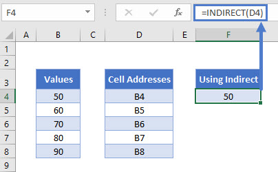

The INDIRECT Function will look at the text string in cell D4 which in this case is B4 – it will then use the text string as a valid cell reference and return the value that is contained in B4 – in this instance, 50.

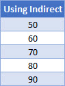
If you copy the formula down, the D4 will change to D5, D6 etc, and the correct value from column B will be returned.

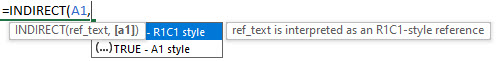
The Syntax of the INDIRECT Function is:

=INDIRECT(reference, reference style)

The reference style can be either R1C1 style or can be the more familiar A1 style.  If you omit this argument, the A1 style is assumed.

SUM Function With the INDIRECT Function

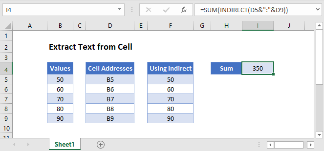
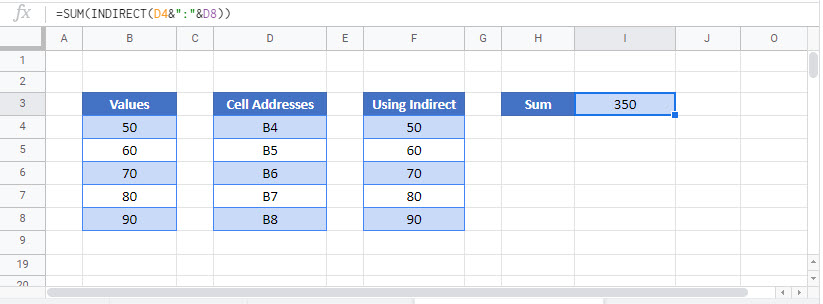
We can also use the INDIRECT function with the SUM Function to add up the values in column B by using the text strings in column D.

Click in H4 and type the following formula.

=SUM(INDIRECT(D4&":"&D8))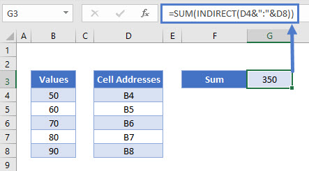

INDIRECT Function With Range Names in Excel

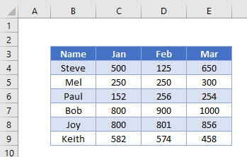
Now let’s look at an example of using the INDIRECT Function with Named Ranges.

Consider the following worksheet where the sales figures are shown for a period of 3 months for several Sales Reps.

1. Select the Range B3:E9.
2. In the Ribbon, select Formulas > Create from Selection.

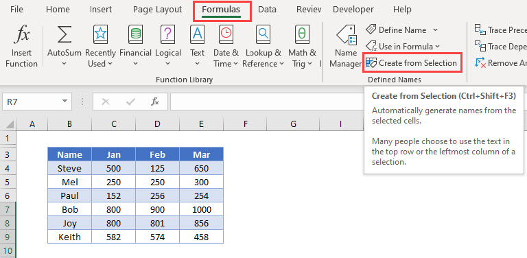
3. Make sure that the Top row and the Left Column check boxes are ticked and click OK.

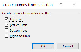
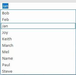
4. Excel will now have created range names based on your selection.

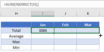
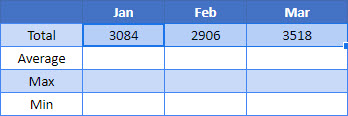
5. Click in H4 and set up a table as shown below.

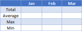
6. In I4, type the following formula:

=SUM(INDIRECT(I3)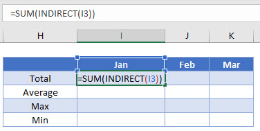

7. Press Enter to complete the formula.

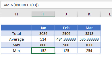
8. Drag the formula across to column K.
9. The formula will change from picking up I3 to picking up J3 (the Feb range name) and then K3 (the March range name).
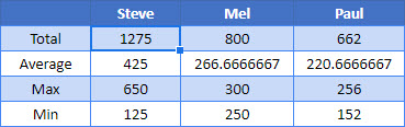
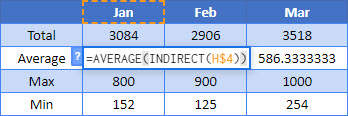
10. Repeat the process for the AVERAGE, MAX and MIN functions.

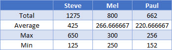
11. We can then amend the names in row 3 to get the totals for 3 of the sales reps. The formulas will automatically pick up the correct values due to the INDIRECT

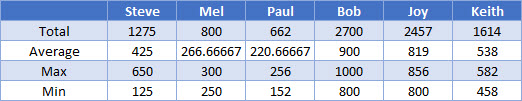
12. Type in the name of the remaining reps in the adjacent column and drag the formulas across to get their sales figures.

 

Cell Value as a Cell Reference in Google Sheets

Using the INDIRECT Function in Google sheets works the same way as it does in Excel.

INDIRECT Function with Range Names in Google Sheets

Named Ranges work similar to Excel in Google Sheets.

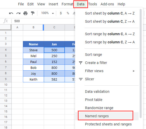
1. In the Menu, select Data>Named Ranges.

2. Type in the name or the range, and then select the range.

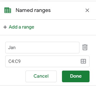
3. Click Done.
4. Repeat the process for all the months, and all the sales reps
5. Once you have created the range names, you can use them in the same way as you used them in Excel.

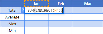
6. Drag the formula across to February and March.

 

7. Repeat for the AVERAGE, MIN and MAX functions.

8. We can then amend the names in row 3 to get the totals for 3 of the sales reps. The formulas will automatically pick up the correct values due to the INDIRECT