VLOOKUP & HLOOKUP Combined – Excel & Google Sheets

This tutorial will demonstrate how to use the VLOOKUP and HLOOKUP Functions together to lookup a value in Excel and Google Sheets.

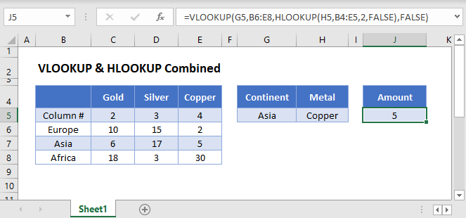
Combine VLOOKUP and HLOOKUP

Sometimes you need the column reference of your VLOOKUP formula to be dynamic. Usually, the best way to do this is by combining the VLOOKUP & MATCH Functions, but in this tutorial we will demonstrate the VLOOKUP-HLOOKUP combination instead.

=VLOOKUP(G3,B4:E6,HLOOKUP(H3,B2:E3,2,FALSE),FALSE)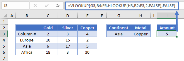

In this example, our formula returns the amount of Copper in Asia, given the continent and the metal.

Let’s see how to combine these two popular functions.

HLOOKUP Function

First add a helper row (Row 3 below) with the column numbers. Then use the HLOOKUP Function to return the column number from that row for use in the VLOOKUP Function.

=HLOOKUP("Copper",B2:E3,2,FALSE)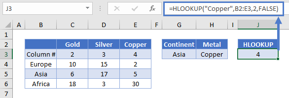

VLOOKUP Function

Once you have the column number, you can use it in your VLOOKUP formula as the col_index_num input.

=VLOOKUP(lookup_value, table_array, col_index_num, [range_lookup])

=VLOOKUP(G3,B4:E6,J3,FALSE)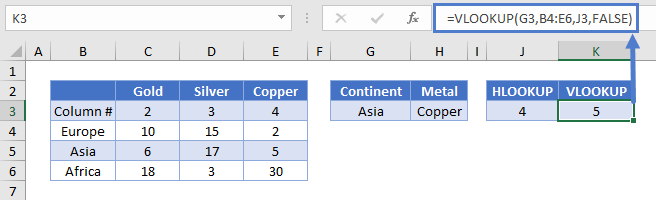

Putting these formulas together, yields our original formula.

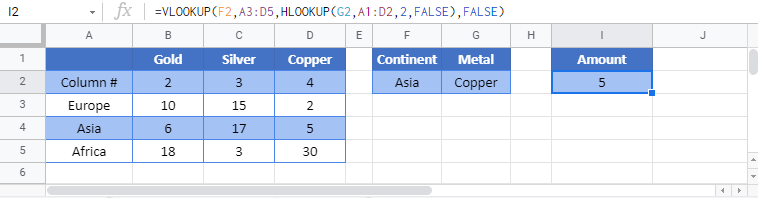
VLOOKUP & HLOOKUP Combined in Google Sheets

All the examples explained above work the same in Google sheets as they do in Excel.