VLOOKUP & MATCH Combined – Excel & Google Sheets
Written by
Reviewed by
Download the example workbook
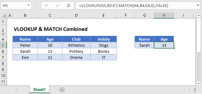
This tutorial will demonstrate how to retrieve data from multiple columns using the MATCH and VLOOKUP Functions in Excel and Google Sheets.
Why Should you Combine VLOOKUP and MATCH?
Traditionally, when using the VLOOKUP Function, you enter a column index number to determine which column to retrieve data from.
This presents two problems:
- If you want to pull values from multiple columns, you must manually enter the column index number for each column
- If you insert or remove columns, your column index number will no longer be valid.
To make your VLOOKUP Function dynamic, you can find the column index number with the MATCH Function.
=VLOOKUP(G3,B3:E5,MATCH(H2,B2:E2,0),FALSE)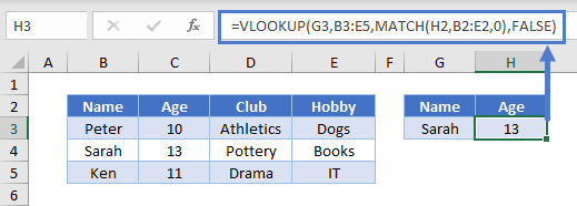
Let’s see how this formula works.
MATCH Function
The MATCH Function will return the column index number of your desired column header.
In the example below, the column index number for “Age” is calculated by the MATCH Function:
=MATCH("Age",B2:E2,0)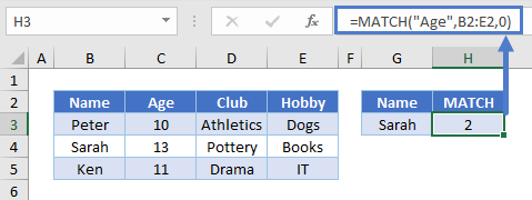
“Age” is the 2nd column header, so 2 is returned.
Note: The last argument of the MATCH Function must be set to 0 to perform an exact match.
VLOOKUP Function
Now, you can simply plug in the result of the MATCH Function into your VLOOKUP Function:
=VLOOKUP(G3,B3:E5,H3,FALSE)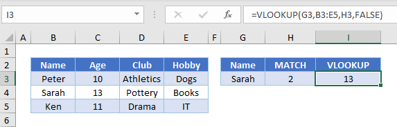
Replacing the column index argument with the MATCH Function gives us our original formula:
=VLOOKUP(G3,B3:E5,MATCH(H2,B2:E2,0),FALSE)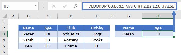
Inserting and Deleting Columns
Now, when you insert or delete columns in the data range, the result of your formula will not change.
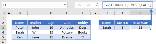
In the example above, we added the Teacher column to the range but still want the student’s Age. The output from the MATCH Function identifies that “Age” is now the 3rd item in the header range, and the VLOOKUP Function uses 3 as the column index.
Locking Cell References
To make our formulas easier to read, we’ve shown the formulas without locked cell references:
=VLOOKUP(G3,B3:E5,MATCH(H2,B2:E2,0),FALSE)But these formulas will not work properly when copy and pasted elsewhere in your file. Instead, you should use locked cell references like this:
=VLOOKUP($G3,$B$3:$E$5,MATCH(H$2,$B$2:$E$2,0),FALSE)Read our article on Locking Cell References to learn more.
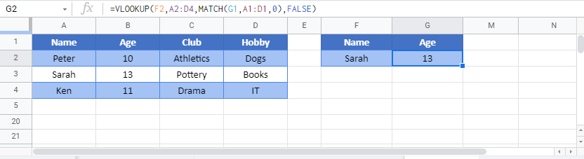
VLOOKUP & MATCH Combined in Google Sheets
These formulas work exactly the same in Google Sheets as in Excel.