VLOOKUP – Multiple Sheets at Once – Excel & Google Sheets

This tutorial will demonstrate how to perform a VLOOKUP on multiple sheets in Excel and Google Sheets. If your version of Excel supports XLOOKUP, we recommend using XLOOKUP instead.

The VLOOKUP Function can only perform a lookup on a single set of data. If we want to perform a lookup among multiple sets of data that are stored in different sheets, we can either combine all sets of data into one set or use the IFERROR Function together with VLOOKUP to perform multiple lookups in a single formula.

The latter method is simpler in Excel while the former is simpler in Google Sheets.

 

VLOOKUP with IFERROR

The VLOOKUP Function (and other lookup formulas) returns an error if it can’t find a match, and we normally use the IFERROR Function to replace the error with a customized value.

Instead of a customized value, we’ll use the IFERROR to perform another VLOOKUP from another sheet if the first VLOOKUP can’t find a match in the first sheet.

VLOOKUP – 2 Sheets at Once

=IFERROR(VLOOKUP(B3,'Department A'!$B$3:$C$7,2,FALSE),VLOOKUP(B3,'Department B'!$B$3:$C$7,2,FALSE))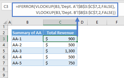

Let’s walkthrough the formula:

 

VLOOKUP Function

Here’s the first VLOOKUP:

=VLOOKUP(B3,'Dept. A'!$B$3:$C$7,2,FALSE)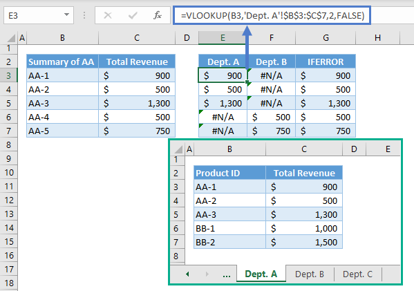

Note: The VLOOKUP Function searches for the lookup value from the first column of the table and returns the corresponding value from the column defined by the column index (i.e., 3^rd argument). The last argument defines the type of match (i.e., True – Approximate Match, False – Exact Match).

Here’s the VLOOKUP for the 2^nd Sheet:

=VLOOKUP(B3,'Dept. B'!$B$3:$C$7,2,FALSE)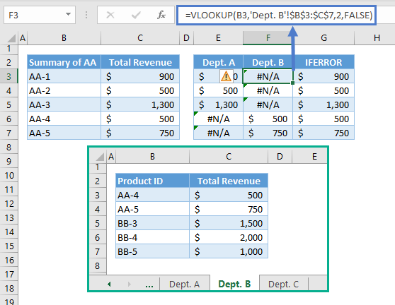

 

IFERROR Function

We combined the results of the 2 VLOOKUPs using the IFERROR Function.

We check the value of the first VLOOKUP (e.g., Department A). If a value is an error, the corresponding value from the 2^nd VLOOKUP is returned instead.

=IFERROR(E3,F3)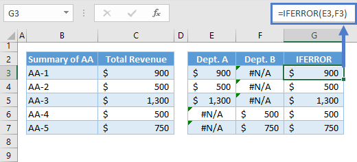

Note: The IFERROR Function checks a value (i.e., 1^st argument) if it’s an error (e.g., #N/A, #REF!). If it’s an error, then it will return the value from its last argument instead of the error. If it’s not an error, it will return the value that is being checked.

 

Combining all these concepts results to our original formula:

=IFERROR(VLOOKUP(B3,'Department A'!$B$3:$C$7,2,FALSE),VLOOKUP(B3,'Department B'!$B$3:$C$7,2,FALSE))

 

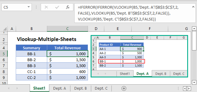
VLOOKUP – More than 2 Sheets at Once

For more than two sheets, we need to add one VLOOKUP and one IFERROR per additional sheet to the formula above. Here’s the formula for 3 sheets:

=IFERROR(IFERROR(VLOOKUP(B3,'Dept. A'!$B$3:$C$7,2,FALSE),VLOOKUP(B3,'Dept. B'!$B$3:$C$7,2,FALSE)),VLOOKUP(B3,'Dept. C'!$B$3:$C$7,2,FALSE))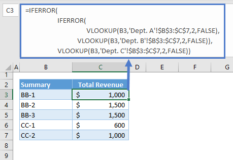

VLOOKUP Multiple Sheets at Once in Google Sheets

Although the combination of IFERROR and VLOOKUP works the same way in Google Sheets, it’s simpler to combine the data sets into one.

 

VLOOKUP with Curly Brackets {} (Google Sheets)

We can combine the data sets into one using the curly brackets.

=VLOOKUP(B3,{'Department A'!$B$3:$C$7;'Department B'!$B$3:$C$7;'Department C'!$B$3:$C$7},2,FALSE)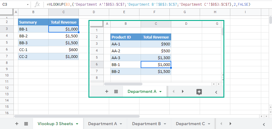

Let’s breakdown and visualize the formula:

Stack all data sets vertically by separating the ranges of cells using the semi-colon inside the curly brackets:

={'Department A'!$B$3:$C$7;'Department B'!$B$3:$C$7;'Department C'!$B$3:$C$7}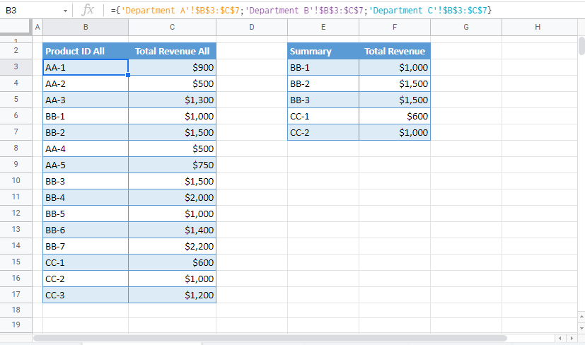

Note: The curly brackets in Google Sheets can also be used to create an array from ranges of cells. The semi-colon is used to stack values vertically while the comma is used to stack values horizontally. If the ranges of cells will be stacked vertically, we need to make sure that the no. of columns for each of the ranges of cells is the same. Otherwise, it won’t work. For horizontal, the no. of rows must be the same.

The resulting array is used as the input for the 2^nd argument of the VLOOKUP:

=VLOOKUP(E3,$B$3:$C$17,2,FALSE)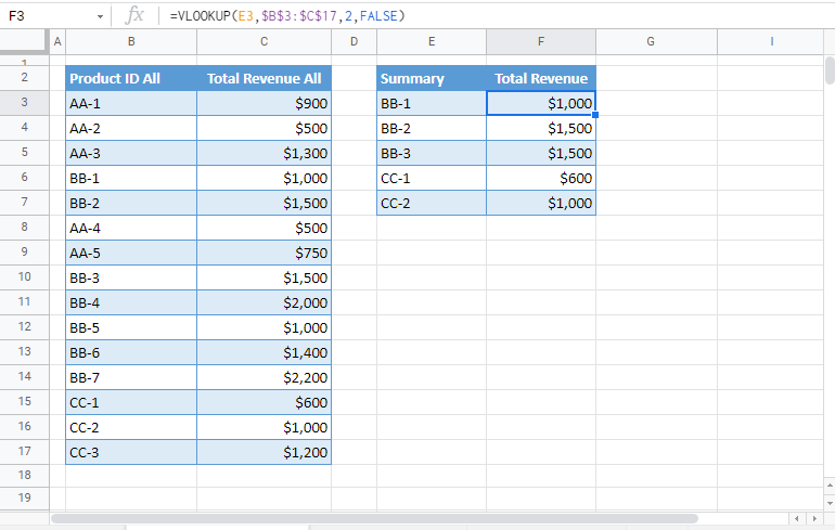

 

Combining all these together results to our original formula:

=VLOOKUP(B3,{'Department A'!$B$3:$C$7;'Department B'!$B$3:$C$7;'Department C'!$B$3:$C$7},2,FALSE)