ADDRESS Function – Get Cell Address – Excel & Google Sheets
Written by
Reviewed by
Download the example workbook
This tutorial demonstrates how to use the ADDRESS Function in Excel and Google Sheets to return a cell address as text.
What is the ADDRESS Function?
The ADDRESS Function Returns a cell address as text.
Usually, in a spreadsheet, we provide a cell reference, and a value from that cell is returned. Instead, the ADDRESS Function builds the name of a cell.
The address can be relative or absolute, in A1 or R1C1 style, and may or may not include the sheet name.
ADDRESS – Basic Example
Let’s say that we want to build a reference to the cell in 4th column and 1st row, aka cell D1. We can use the layout pictured here:
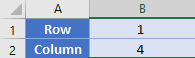
Our formula in A3 is simply
=ADDRESS(B1, B2)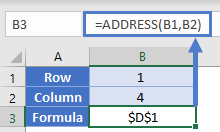
Note: By default the ADDRESS Function returns an absolute cell reference. By updating an optional argument we can change the cell references from absolute to relative. Let’s review this and other inputs to the ADDRESS Function…
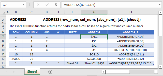
ADDRESS Function Syntax and Inputs:
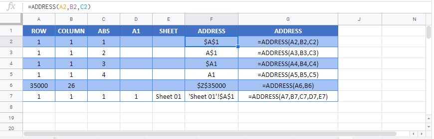
=ADDRESS(row_num,column_num,abs_num,C1,sheet_text)row_num – The row number for the reference. Example: 5 for row 5.
col_num – The column number for the reference. Example: 5 for Column E. You can not enter “E” for column E
abs_num – [optional] A number representing if the reference should have absolute or relative row/column references. 1 for absolute. 2 for absolute row/relative column. 3 for relative row/absolute column. 4 for relative.
a1 – [optional]. A number indicating whether to use standard (A1) cell reference format or R1C1 format. 1/TRUE for Standard (Default). 0/FALSE for R1C1.
sheet_text – [optional] The name of the worksheet to use. Defaults to current sheet.
ADDRESS with INDIRECT
We can combine ADDRESS with the INDIRECT Function. Consider this layout, where we have a list of items in column D.
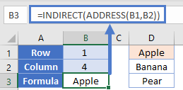
We can generate a reference to D1 like so
=ADDRESS(B1, B2)
=$D$1
By putting the address function inside an INDIRECT function, we’ll be able to use the generated cell reference and use it in a practical way. The INDIRECT will take the reference of “$D$1” and use it to fetch the value from that cell.
=INDIRECT(ADDRESS(B1, B2)
=INDIRECT($D$1)
="Apple"
Note: While the above gives a good example of making the ADDRESS Function useful, it’s not a good formula to use normally. It required two functions, and because of the INDIRECT it will be volatile in nature. A better alternative would have been to use the INDEX Function like this:
=INDEX(1:1048576, B1, B2)
Address of Specific Value
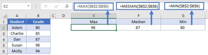
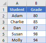
Sometimes when you have a large list of items, you need to know the location of an item in the list. Consider this table of scores from students. We’ve gone ahead and calculated the min, median, and max values of these scores in cells E2:G2.
Let’s say we wanted to find these values. We have a two options:
- Filter our table for each of these items.
- Use the MATCH Function with ADDRESS. Remember that MATCH will return the relative position of a value within a range.
Our formula in E3 then is:
=ADDRESS(MATCH(E2, $B:$B, 0), 2)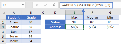
We can copy this same formula across to G3, and only the E2 reference will change since it’s the only relative reference. Looking back at E3, the MATCH function was able to find the value of 98 in the 5th row of column B. Our ADDRESS function then used this to build the full address of “$B$5”.
Translate Column Letters from Numbers
So far, all of the examples have returned an absolute reference. Let’s return a relative reference instead.
Below, in column B, we want to calculate the column letter corresponding to the column number in column A.
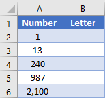
We will use the ADDRESS Function to return a reference on row 1 in relative format, and then we’ll remove the “1” from the text string so that we just have the letter(s) left. Consider in our table row 3, where our input is 13. Our formula in B3 is
=SUBSTITUTE(ADDRESS(1, A3, 4), "1", "")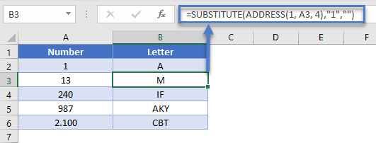
Note that we’ve given the 3rd argument within the ADDRESS function, which controls the relative vs. absolute referencing. The ADDRESS function will output “M1”, and then the SUBSTITUTE function removes the “1” so that we are left with just the “M”.
Find the Address of Named Ranges
In Excel, you can name range or ranges of cells, allowing you to simply refer to the named range instead of the cell reference.
Most named ranges are static, meaning they always refer to the same range. However, you can also create dynamic named ranges that change in size based on some formula(s).
With a dynamic named range, you might need to know the exact address that your named range is pointing to. We can do this with the ADDRESS Function.
In this example, we’ll look at how to define the address for our named range called “Grades”.
Let’s bring back our table from before:
To get the address of a range, you need to know the top left cell and the bottom left cell. The first part is easy enough to accomplish with the help of the ROW and COLUMN functions. Our formula in E1 can be
=ADDRESS(ROW(Grades), COLUMN(Grades))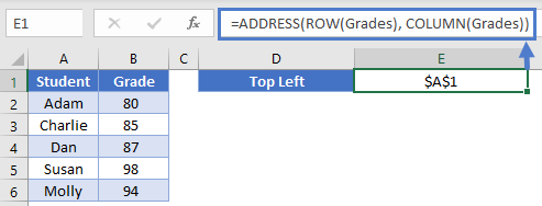
The ROW Function returns the row of the first cell in our range (which will be 1), and the COLUMN will do the same similarly for the column (also 1).
This formula will get the bottom-right cell
=ADDRESS(ROWS(Grades)-ROW(Grades)+1, COLUMNS(Grades)-COLUMN(Grades)+1)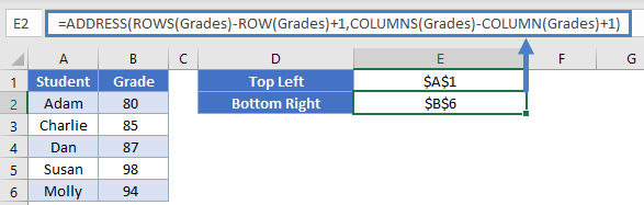
We used the ROWS and COLUMNS functions to calculate the height and width of the range. By subtracting the first row and column numbers, we calculate the last cell in the range
Finally, to put it all together into a single string, we can simply concatenate the values together with a colon in the middle. Formula in E3 can be
=E1 & ":" & E2
Note: While we were able to determine the address of the range, our ADDRESS function determined whether to list the references as relative or absolute. Your dynamic ranges will have relative references that this technique won’t pick up.
2nd Note: This technique only works on a continuous names range. If you had a named range that was defined as something like this formula
=A1:B2, A5:B6then the technique above would result in errors.
ADDRESS function in Google Sheets
The ADDRESS function works exactly the same in Google Sheets as in Excel.