How to Filter by Color in Excel & Google Sheets
Written by
Reviewed by
Last updated on September 5, 2022
In this tutorial, you will learn how to filter data by color in Excel and Google Sheets.
Filter by Color
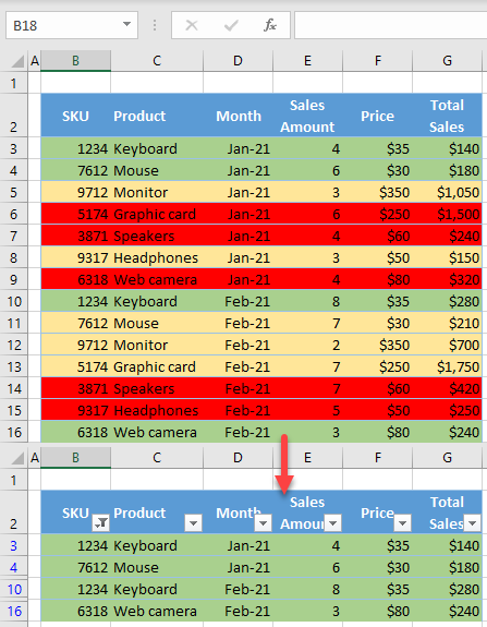
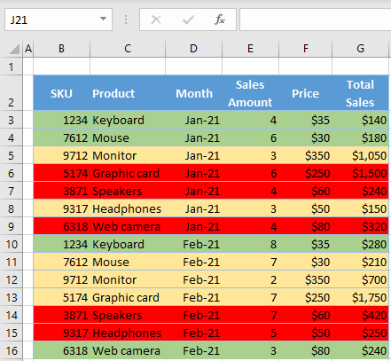
Say you have the formatted data set shown below and want to filter and only display those rows highlighted in green.
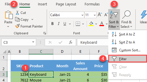
- First, turn on the filter. Click anywhere in the data range (e.g., B2:G16) and in the Ribbon, go to Home > Sort & Filter > Filter.
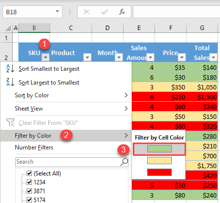
- Click on the filter button next to any of the column headings (B2, for example), go to Filter by Color, and choose green.
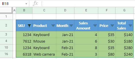
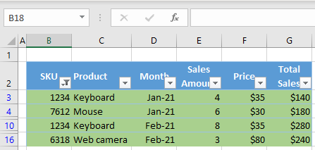
As a result, only rows with cells colored in green are displayed (3, 4, 10, and 16) while all other rows are hidden.
Filter by Color in Google Sheets
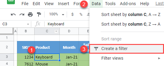
- To create a filter, click anywhere in the data range (B2:G16) and in the Menu, go to Data > Create a filter.
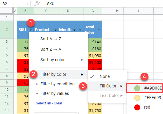
- Click on the filter button next to any of the column headings (B2, for example). Then go to Filter by color > Fill Color and choose green (#A9D08E).
The result is the same as in Excel: All green rows are displayed.